Chapter 2 An Overview of Statistical Learning
2.1 Conceptual Exercises
2.1.1 Exercise 1.
This exercise is about flexible and inflexible statistical learning methods. First, let’s recall what are the differences between these methods. The aim of statistical learning is to estimate a function \(f\) such that \(f\) is a link between the input \(X\) and the output \(Y\). A flexible model means that we do not assume a particular form for \(f\). So, an advantage of such models is to generally provide a better fit to the data (however, be careful with the overfitting) but the number of parameters to estimate is usually large. At the contrary, an inflexible model has less parameters but we have to prespecified a particular form for the data (for example linear), even if it poorly fits the data.
- Question (a)
The case of sample size \(n\) extremely large and number of predictors \(p\) small is the ideal case in statistical learning. A flexible method should perform very well in this case. The flexible method will tend to reduce the bias and won’t be too sensitive to the noise thanks to the large size of the sample.
- Question (b)
The case of sample size \(n\) small and number of predictors \(p\) very large refers to the high dimensional settings. An inflexible method should show better performance than a flexible one in this case. Here, the trade-off between bias and variance is very important. We allow some bias by using an inflexible model with the hope to reduce a lot the noise in the data.
- Question (c)
In the case of highly non-linear relationship between predictors and reponse, a flexible model will perform better than an inflexible one. In case of inflexible model, we set a particular form for \(f\) and we usually can not specified a function for \(f\) if \(f\) is highly non-linear.
- Question (d)
If the variance of the error terms is extremely high, an inflexible model will perform better than a flexible one. Because, if we set a flexible method, the function \(f\) will tend to follow the error and thus will overfit.
2.1.2 Exercise 2.
This exercise is about the difference between regression and classification problems and the inference or prediction purposes. Let’s recall what these different terms mean. A regression task is done when we try to infer or predict an output which takes continuous values. A classification task is done when we try to infer or predict an output which takes discrete values. An inference purpose consists in the understanding of how the features have an influence on the response, whereas a prediction purpose is to find a value of the output variable based on a new realisation of the dependant variables and the knowledge of some features and outputs.
- Question (a)
This is a regression problem because the CEO salary is a continuous variable. We aim to do inference here (understanding which factors). \(n\) is equal to 500 (top 500 firms in the US), \(p\) equals to 3 (profit, number of employees and industry) and the output is the CEO salary.
- Question (b)
This is a classification problem because the output varible is discrete (success or failure). We aim to do prediction (launching a new product and wish to know whether it will be a success or a failure). \(n\) is equal to 20, \(p\) equals to 13 (price charged for the product, marketing budget, competition price, and ten other variables) and the output variable is success or failure.
- Question (c)
This is a regression problem because the % change in the US dollar is continuous. We aim to do prediction (We are interesting in predicting). \(n\) is equal to 52 (number of week in 2012), \(p\) equals to 3 (the % change in the US market, the % change in the British market, and the % change in the German market) and the output variable is the % change in the dollar.
2.1.3 Exercise 3.
This exercise is about the bias-variance decomposition of the mean square error.
Consider the following model: \(y = f(x) + \epsilon\). We denote by \(\widehat{y}\) and \(\widehat{f}\) the estimation of \(y\) and \(f\). The mean square error is:
\[MSE = \mathbb{E}\left[(\widehat{y} - y)^2\right].\]
As a more complex model leads to a better estimation of the function \(f\), the training error decreases as the model complexity increases. The MSE can be decomposed into three terms: variance, squared bias and irreducible error. “Variance refers to the amount by which \(\widehat{f}\) would change if we estimated it using a different training data set.” So, the variance increases with the model complexity because a complex model is very flexible and gives a different function for each training data set. Conversely, the bias decreases with the model complexity because such a model will fit perfectly the data. The irreducible error is equal to \(Var(\epsilon)\). The test error has a U-shape because it is the sum of the three previous curves.
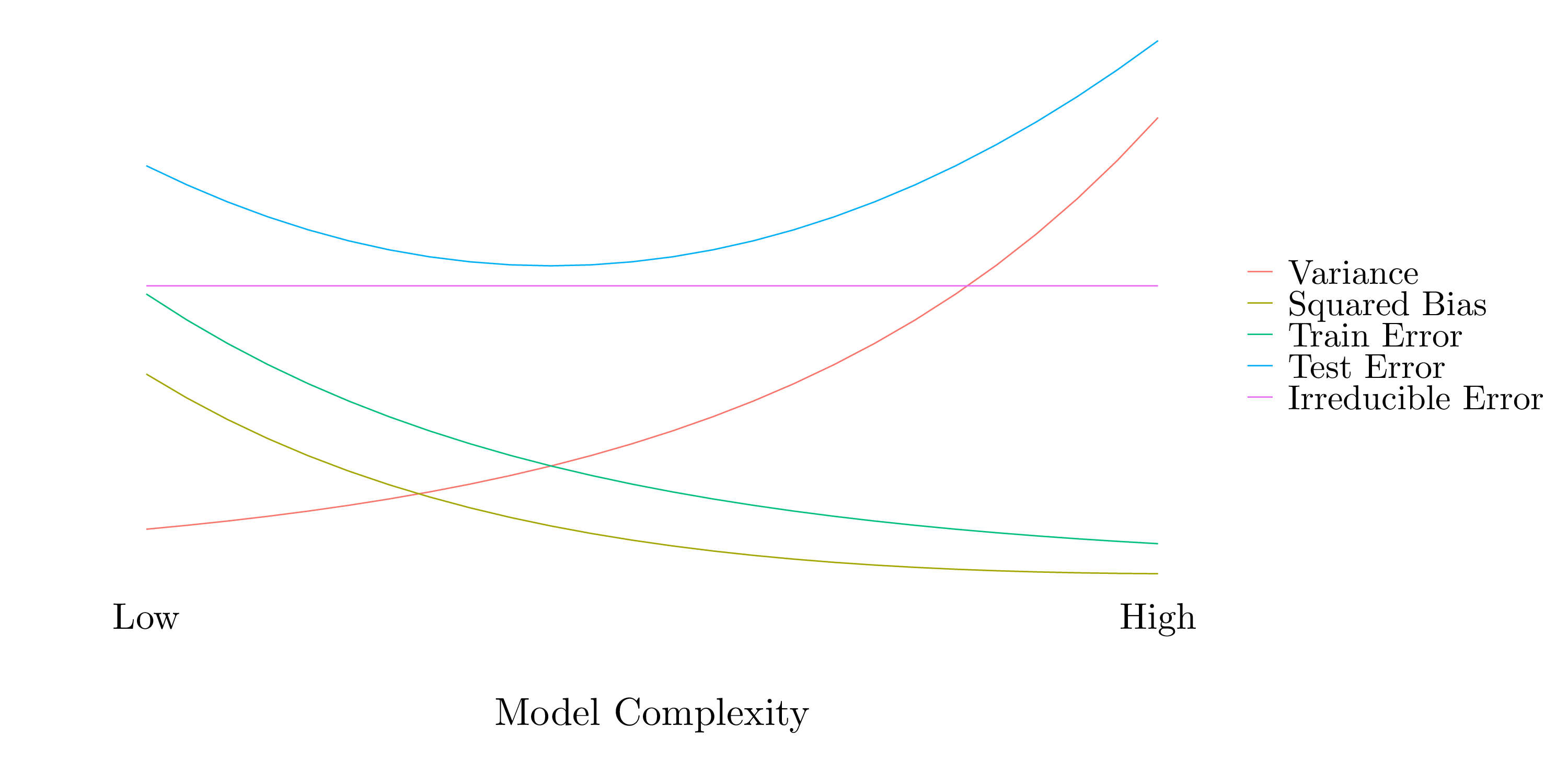
Figure 2.1: Model complexity.
2.1.4 Exercise 4.
This exercise is about giving examples of real-life applications of statistical learning.

From Armando Arroyo GeekStyle on Linkedin.
2.1.5 Exercise 5.
This exercise is about the difference between flexible and non-flexible statistical learning methods.
A very flexible method has for main advantage over a less flexible methods the large number of functional forms that it can take. It shows two majors drawbacks: the first one is the number of parameters to fit (usually, way more larger than the non-flexible methods) and the second one, its propension to overfit the data. Moreover, they can exhibit less interpretability.
We can prefer a less flexible approach when we want to do inference of the dataset because of the interpretability of such models. However, when the goal is prediction, we may use very flexible methods in order to (hopefully) have better results. The choice of between a very flexible and a less flexible method refers closely with the bias-variance tradeoff. In general, a very flexible one will lead to small bias, large variance and a less flexible one to large bias, small variance.
2.1.6 Exercise 6.
This exercise is about the difference between parametric and non-parametric approaches.
Consider the following model: \(Y = f(X) + \epsilon\). We aim to estimate the function \(f\). For the parametric approaches, we assume a particular form for \(f\), linear for example, and then, estimate some parameters. However, if the form we assume is not the right one, our estimate won’t be very accurate. At the opposite, non-parametric approaches do not assume a particular form for \(f\). So, the estimate of \(f\) will be close to the true functional form of \(f\). But, we need a lot of data (compare to parametric approches) to obtain an accurate estimate of \(f\).
2.1.7 Exercise 7.
This exercise is an application of \(K\)-nearest neighbors.
| Obs | \(X_1\) | \(X_2\) | \(X_3\) | \(Y\) |
|---|---|---|---|---|
| 1 | 0 | 3 | 0 | Red |
| 2 | 2 | 0 | 0 | Red |
| 3 | 0 | 1 | 3 | Red |
| 4 | 0 | 1 | 2 | Green |
| 5 | -1 | 0 | 1 | Green |
| 6 | 1 | 1 | 1 | Red |
- Question (a)
The euclidean distance between to two \(n\)-dimensional vectors \(X\) and \(Y\) is defined by \[ d(X, Y) = \sqrt{\sum_{i = 1}^n (X_i - Y_i)^2}\]
| Obs | 1 | 2 | 3 | 4 | 5 | 6 |
|---|---|---|---|---|---|---|
| \(d(0/i)\) | 3 | 2 | \(\sqrt{10}\) | \(\sqrt{5}\) | \(\sqrt{2}\) | \(\sqrt{3}\) |
- Question (b)
For \(K = 1\), we classify the test point where the closest observation is. The closest point is the point 5, so the test point will be Green.
- Question (c)
For \(K = 3\), we classify the test point where the three closest observation are. The three closest points are the 2, 5 and 6. Two points are red and one is green, so the test point will be Red.
- Question (d)
If the Bayes decision boundary in this problem is highly non-linear, we would expect the best value for K to be small because the smaller \(K\) is, the more flexible the model is. So, if the model is very flexible, it will adapt to highly non-linear problem.
2.2 Applied Exercises
2.2.1 Exercise 8.
This exercise is about the College dataset. It contains 777 observations of 18 variables about the universities and colleges in the United States. For a description of the variables, please refer to the page 54 of the book or in R by typing help(College) after loading the package ISLR.
- Question (a) and (b)
- Question (c) i
- Factor variables
- Private
|
- Numeric variables
| Name | NA_num | Unique | Range | Mean | Variance | Minimum | Q05 | Q10 | Q25 | Q50 | Q75 | Q90 | Q95 | Maximum |
|---|---|---|---|---|---|---|---|---|---|---|---|---|---|---|
| Apps | 0 | 711 | 48013.0 | 3001.64 | 14978459.53 | 81.0 | 329.8 | 457.6 | 776.0 | 1558.0 | 3624.0 | 7675.0 | 11066.2 | 48094.0 |
| Accept | 0 | 693 | 26258.0 | 2018.80 | 6007959.70 | 72.0 | 272.4 | 361.6 | 604.0 | 1110.0 | 2424.0 | 4814.2 | 6979.2 | 26330.0 |
| Enroll | 0 | 581 | 6357.0 | 779.97 | 863368.39 | 35.0 | 118.6 | 154.0 | 242.0 | 434.0 | 902.0 | 1903.6 | 2757.0 | 6392.0 |
| Top10perc | 0 | 82 | 95.0 | 27.56 | 311.18 | 1.0 | 7.0 | 10.0 | 15.0 | 23.0 | 35.0 | 50.4 | 65.2 | 96.0 |
| Top25perc | 0 | 89 | 91.0 | 55.80 | 392.23 | 9.0 | 25.8 | 30.6 | 41.0 | 54.0 | 69.0 | 85.0 | 93.0 | 100.0 |
| F.Undergrad | 0 | 714 | 31504.0 | 3699.91 | 23526579.33 | 139.0 | 509.8 | 641.0 | 992.0 | 1707.0 | 4005.0 | 10024.4 | 14477.8 | 31643.0 |
| P.Undergrad | 0 | 566 | 21835.0 | 855.30 | 2317798.85 | 1.0 | 20.0 | 35.0 | 95.0 | 353.0 | 967.0 | 2016.6 | 3303.6 | 21836.0 |
| Outstate | 0 | 640 | 19360.0 | 10440.67 | 16184661.63 | 2340.0 | 4601.6 | 5568.8 | 7320.0 | 9990.0 | 12925.0 | 16552.8 | 18498.0 | 21700.0 |
| Room.Board | 0 | 553 | 6344.0 | 4357.53 | 1202743.03 | 1780.0 | 2735.8 | 3051.2 | 3597.0 | 4200.0 | 5050.0 | 5950.0 | 6382.0 | 8124.0 |
| Books | 0 | 122 | 2244.0 | 549.38 | 27259.78 | 96.0 | 350.0 | 400.0 | 470.0 | 500.0 | 600.0 | 700.0 | 765.6 | 2340.0 |
| Personal | 0 | 294 | 6550.0 | 1340.64 | 458425.75 | 250.0 | 500.0 | 600.0 | 850.0 | 1200.0 | 1700.0 | 2200.0 | 2488.8 | 6800.0 |
| PhD | 0 | 78 | 95.0 | 72.66 | 266.61 | 8.0 | 43.8 | 50.6 | 62.0 | 75.0 | 85.0 | 92.0 | 95.0 | 103.0 |
| Terminal | 0 | 65 | 76.0 | 79.70 | 216.75 | 24.0 | 52.8 | 59.0 | 71.0 | 82.0 | 92.0 | 96.0 | 98.0 | 100.0 |
| S.F.Ratio | 0 | 173 | 37.3 | 14.09 | 15.67 | 2.5 | 8.3 | 9.9 | 11.5 | 13.6 | 16.5 | 19.2 | 21.0 | 39.8 |
| perc.alumni | 0 | 61 | 64.0 | 22.74 | 153.56 | 0.0 | 6.0 | 8.0 | 13.0 | 21.0 | 31.0 | 40.0 | 46.0 | 64.0 |
| Expend | 0 | 744 | 53047.0 | 9660.17 | 27266865.64 | 3186.0 | 4795.8 | 5558.2 | 6751.0 | 8377.0 | 10830.0 | 14841.0 | 17974.8 | 56233.0 |
| Grad.Rate | 0 | 81 | 108.0 | 65.46 | 295.07 | 10.0 | 37.0 | 44.6 | 53.0 | 65.0 | 78.0 | 89.0 | 94.2 | 118.0 |
- Question (c) ii
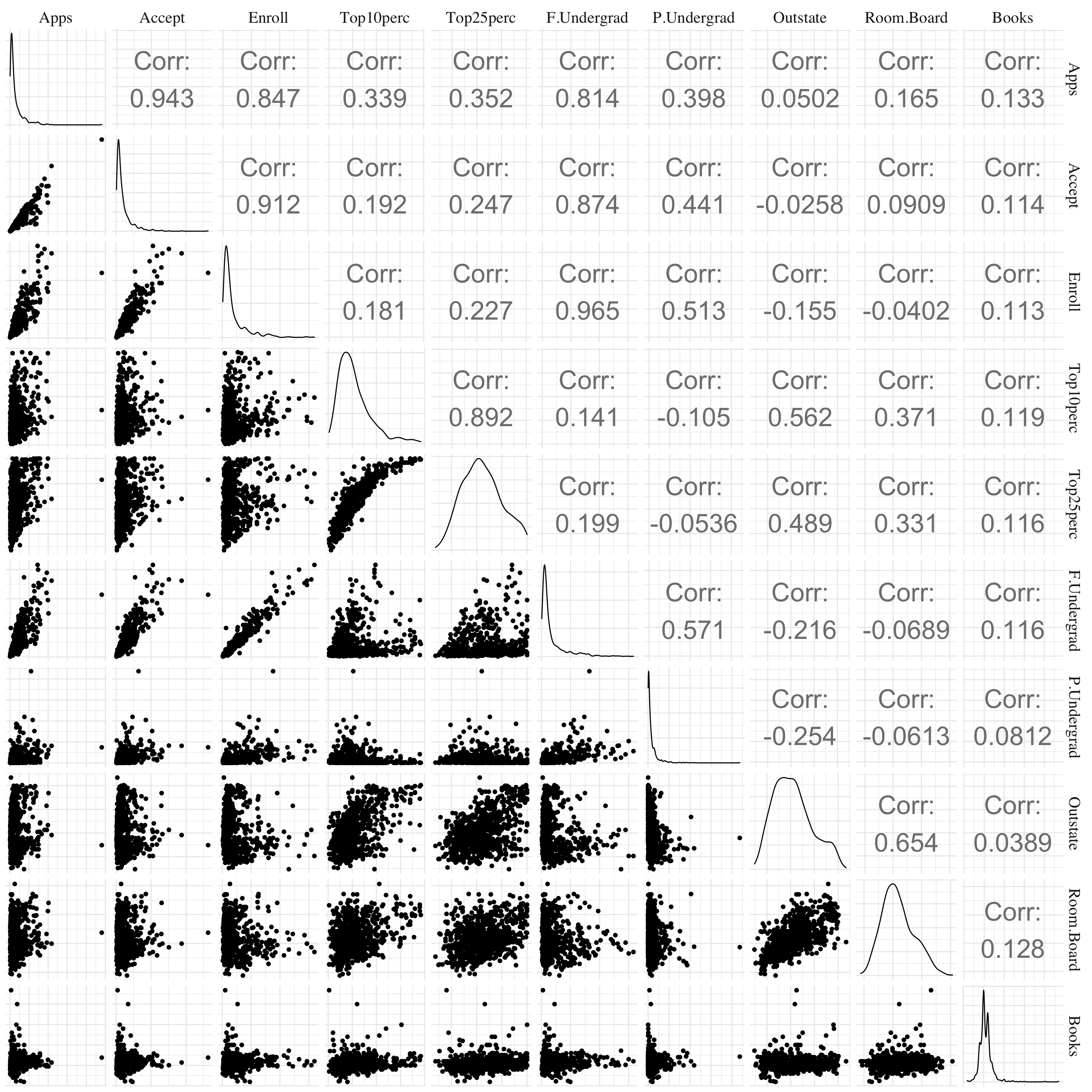
Figure 2.2: Pair plots.
- Question (c) iii
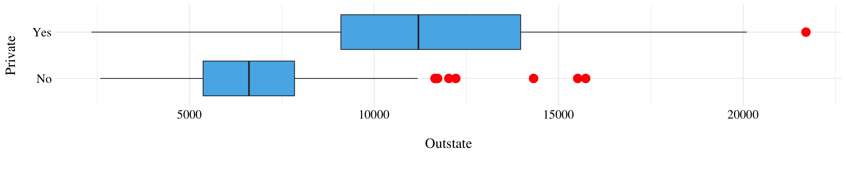
Figure 2.3: Boxplots of the variable Outstate by Private.
- Question (c) iv
- Factor variables
- Elite
|
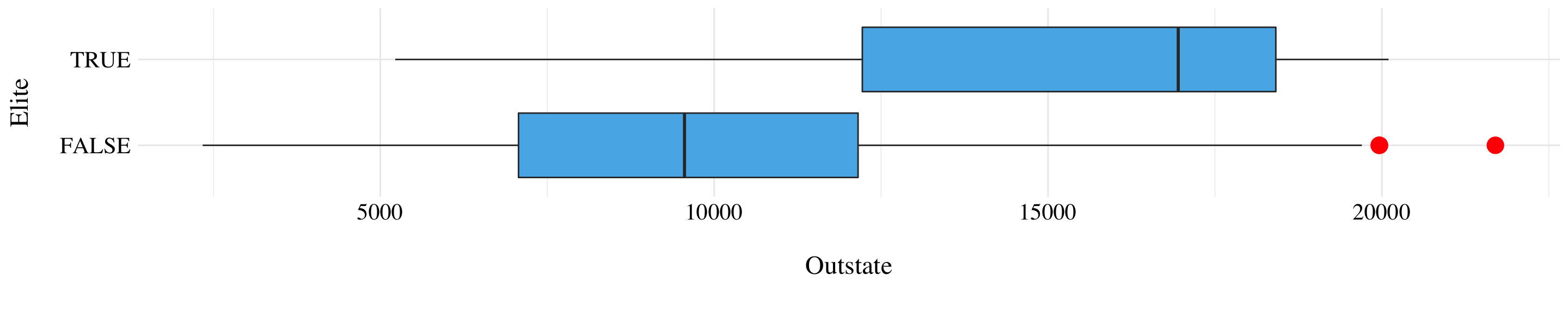
Figure 2.4: Boxplots of the variable Outstate vs Elite.
- Question (c) v
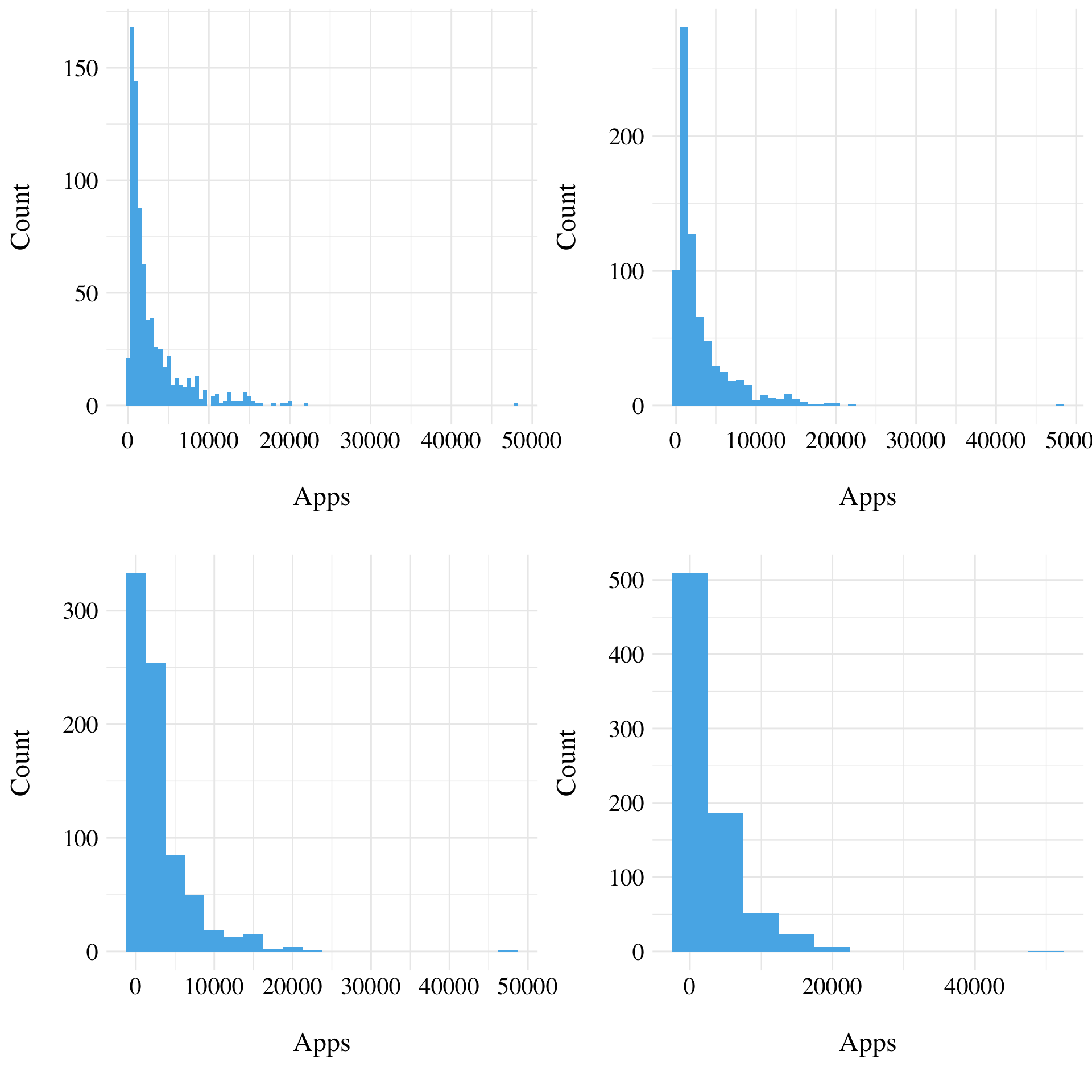
Figure 2.5: Histograms of the variable Apps for different binwidth.
- Question (c) vi
As a brief summary, we found that there is a huge correlation between the number of full-time undergraduates and the number of applications received, accepted and students enrolled. The price to be enrolled in a private university is in mean twice as the price for a public one. But the variance of the price for the private colleges is very important. Moreover, the maximum value of the price for public universities is almost equal to the mean of the private ones (except outliers). Finally, the elite universities (the ones with new students from top 10% of high school class) are usually more expensive than the other ones.
2.2.2 Exercise 9.
This exercise is about the Auto dataset. It contains 392 observations of 9 variables about vehicles. For a description of the variables, please refer to R by typing help(Auto) after loading the package ISLR.
Auto <- as_tibble(Auto, rownames = NA)
Auto <- Auto %>% select(-name) %>%
mutate(cylinders = as.factor(cylinders), year = as.factor(year), origin = as.factor(origin))- Question (a), (b) and (c)
- Factor variables
- cylinders
- year
- origin
|
|
|
- Numeric variables
| Name | NA_num | Unique | Range | Mean | Variance | Minimum | Q05 | Q10 | Q25 | Q50 | Q75 | Q90 | Q95 | Maximum |
|---|---|---|---|---|---|---|---|---|---|---|---|---|---|---|
| mpg | 0 | 127 | 37.6 | 23.45 | 60.92 | 9 | 13.000 | 14 | 17.000 | 22.75 | 29.000 | 34.19 | 37.000 | 46.6 |
| displacement | 0 | 81 | 387.0 | 194.41 | 10950.37 | 68 | 85.000 | 90 | 105.000 | 151.00 | 275.750 | 350.00 | 400.000 | 455.0 |
| horsepower | 0 | 93 | 184.0 | 104.47 | 1481.57 | 46 | 60.550 | 67 | 75.000 | 93.50 | 126.000 | 157.70 | 180.000 | 230.0 |
| weight | 0 | 346 | 3527.0 | 2977.58 | 721484.71 | 1613 | 1931.600 | 1990 | 2225.250 | 2803.50 | 3614.750 | 4277.60 | 4464.000 | 5140.0 |
| acceleration | 0 | 95 | 16.8 | 15.54 | 7.61 | 8 | 11.255 | 12 | 13.775 | 15.50 | 17.025 | 19.00 | 20.235 | 24.8 |
- Question (d)
- Factor variables
- cylinders
- year
- origin
|
|
|
- Numeric variables
| Name | NA_num | Unique | Range | Mean | Variance | Minimum | Q05 | Q10 | Q25 | Q50 | Q75 | Q90 | Q95 | Maximum |
|---|---|---|---|---|---|---|---|---|---|---|---|---|---|---|
| mpg | 0 | 125 | 35.6 | 24.40 | 61.89 | 11.0 | 13.0 | 15.0 | 18.00 | 23.95 | 30.55 | 35.4 | 37.775 | 46.6 |
| displacement | 0 | 70 | 387.0 | 187.24 | 9935.78 | 68.0 | 85.0 | 90.0 | 100.25 | 145.50 | 250.00 | 350.0 | 360.000 | 455.0 |
| horsepower | 0 | 84 | 184.0 | 100.72 | 1275.12 | 46.0 | 60.0 | 65.0 | 75.00 | 90.00 | 115.00 | 150.0 | 170.000 | 230.0 |
| weight | 0 | 279 | 3348.0 | 2935.97 | 658208.03 | 1649.0 | 1934.0 | 1985.0 | 2213.75 | 2792.50 | 3508.00 | 4177.5 | 4391.250 | 4997.0 |
| acceleration | 0 | 92 | 16.3 | 15.73 | 7.26 | 8.5 | 11.4 | 12.5 | 14.00 | 15.50 | 17.30 | 19.0 | 20.475 | 24.8 |
- Question (e)
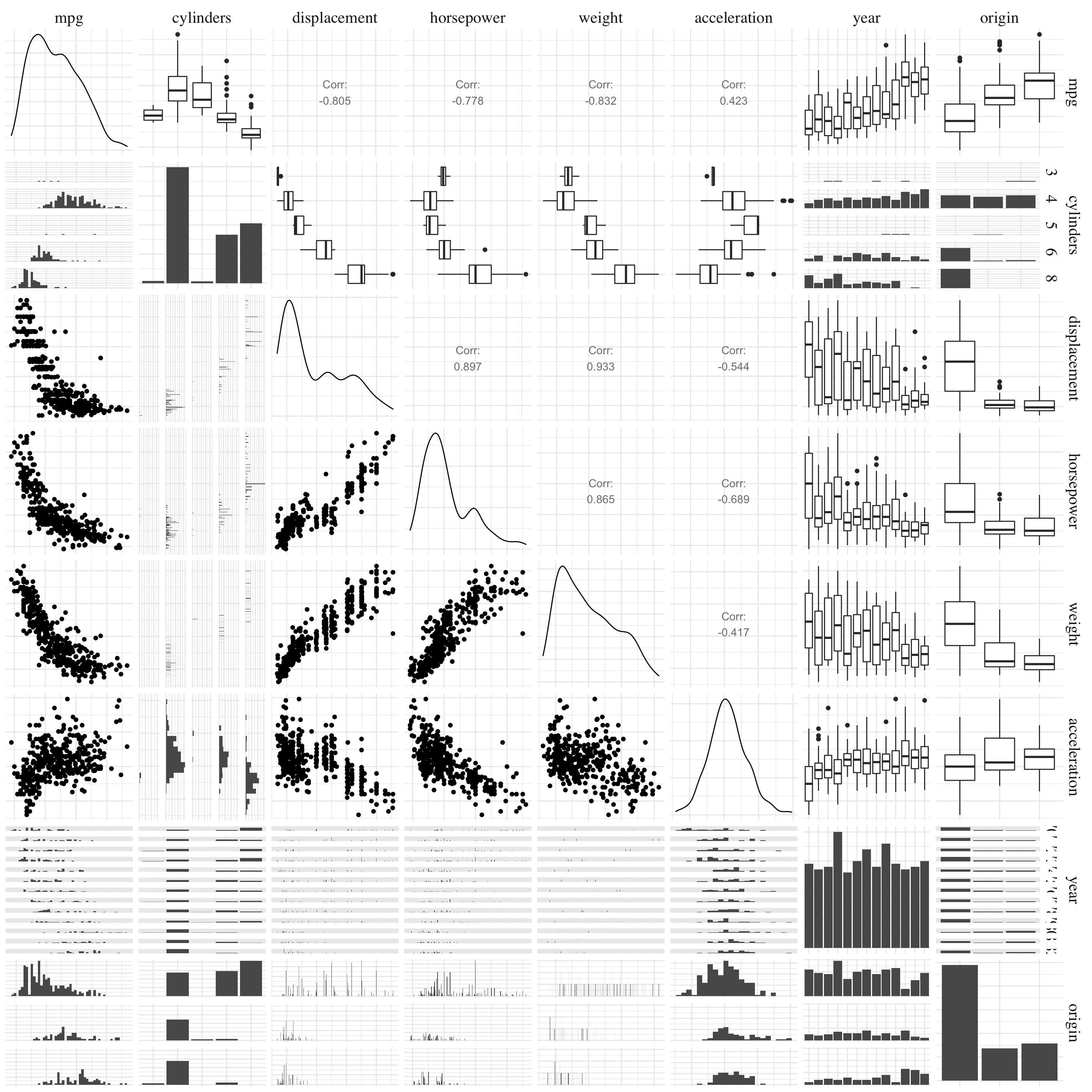
Figure 2.6: Pairs plot
- Question (f)
The variables displacement, weight and origin have a huge correlation with the variable to predict, mpg. So, this ones could particularly useful for the prediction. The relation between these variables does not seem to be linear but instead in \(\exp(-x)\). Moreover, the miles per gallon look very different depending on the origin of the car.
2.2.3 Exercise 10.
This exercise is about the Boston dataset.
- Question (a)
Boston <- as_tibble(Boston, rownames = NA)
Boston <- Boston %>% mutate(chas = as.logical(chas), rad = as.factor(rad))
It contains 506 observations of 14 variables about housing values in suburbs of Boston. Each of the observation represents a suburb of Boston. For a description of the variables, please refer to R by typing help(Boston) after loading the package MASS.
- Question (b)
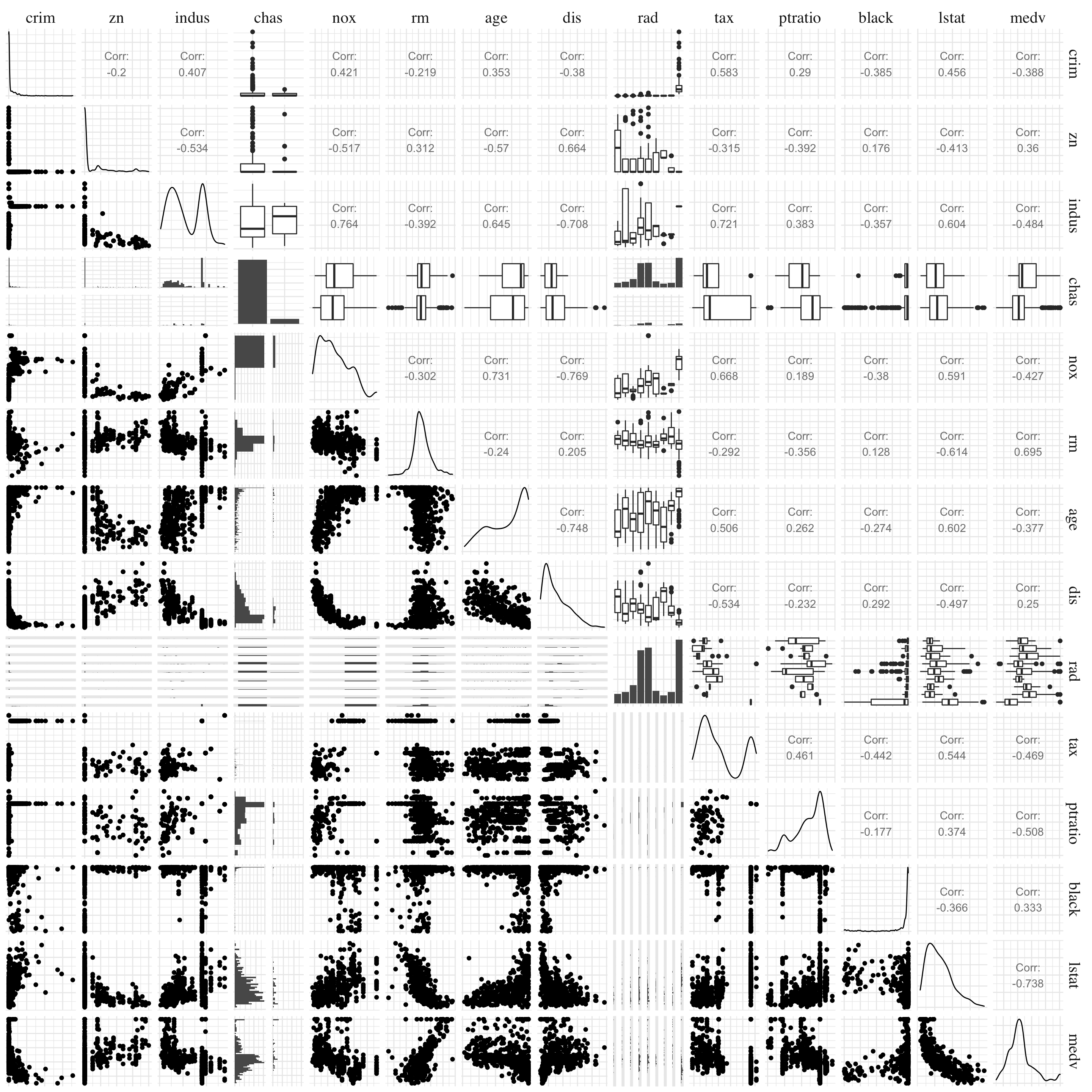
Figure 2.7: Pairs plot
We can see some interesting correlations in this dataset. For exemple, the mean distances to five Boston employement has a correlation of -0.77 with the nitrogen oxides concentration. Or, the lower status of the population are related to the average number of rooms per dwelling (-0.61 for correlation). The variable that are the most related with the crime rate by town is the full-value property-tax rate per $10,000.
- Question (c)
The variable crim seems to be associated with the variables tax, lstat and nox because they have quite a large correlation with the variable of interest (cf. previous question).
- Question (d)
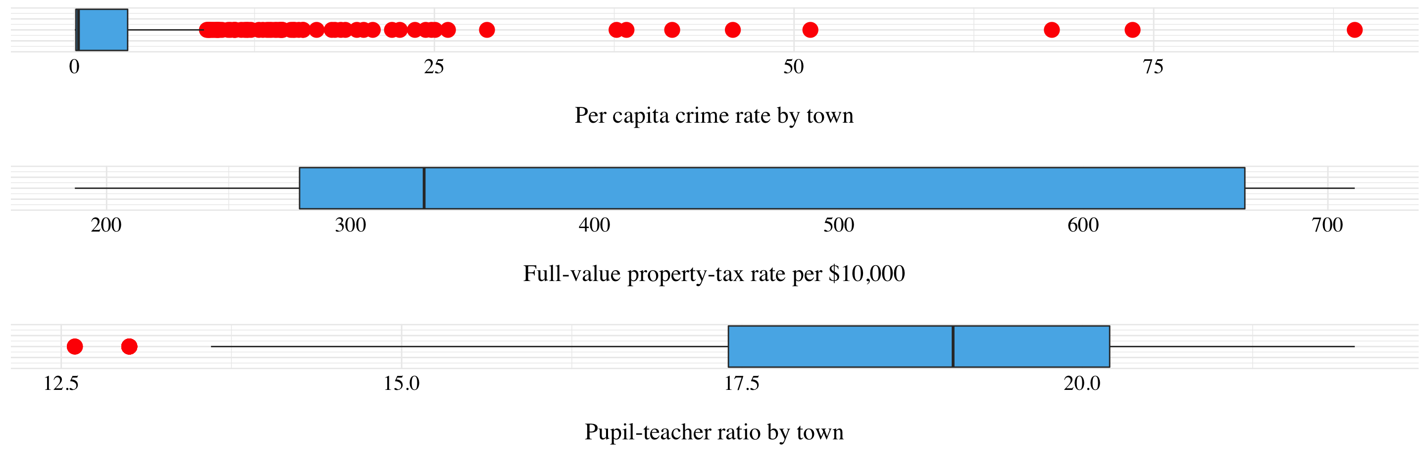
Figure 2.8: Boxplots of some variables.
Half of the suburbs have less than 10% of crime rates, but for three of them, this rate is greater than 70%. The range for this variable is very important. The tax rates do not seem to have outliers but the range is also very important. Indeed, the tax can go from under $200,000 to above $700,000. Finally, there are some suburbs in Boston that have a very low pupil-teacher ratio compare to the others. However, the range is not very wide.
- Question (e)
There are 35 suburbs that bound the Charles river.
- Question (f)
The median pupil-teacher ratio among the towns of Boston is 19.05%.
- Question (g)
| crim | zn | indus | chas | nox | rm | age | dis | rad | tax | ptratio | black | lstat | medv |
|---|---|---|---|---|---|---|---|---|---|---|---|---|---|
| 38.3518 | 0 | 18.1 | FALSE | 0.693 | 5.453 | 100 | 1.4896 | 24 | 666 | 20.2 | 396.90 | 30.59 | 5 |
| 67.9208 | 0 | 18.1 | FALSE | 0.693 | 5.683 | 100 | 1.4254 | 24 | 666 | 20.2 | 384.97 | 22.98 | 5 |
Two suburbs share the lowest median value of owner-occupied homes in $1000s. They have pretty the same values for the other predictors (except maybe for the crime rate).
- Question (h)
There are 64 suburbs with an average of number of rooms per dwelling larger than 7 and 13 with more than 8.
| crim | zn | indus | chas | nox | rm | age | dis | rad | tax | ptratio | black | lstat | medv |
|---|---|---|---|---|---|---|---|---|---|---|---|---|---|
| 0.12083 | 0 | 2.89 | FALSE | 0.4450 | 8.069 | 76.0 | 3.4952 | 2 | 276 | 18.0 | 396.90 | 4.21 | 38.7 |
| 1.51902 | 0 | 19.58 | TRUE | 0.6050 | 8.375 | 93.9 | 2.1620 | 5 | 403 | 14.7 | 388.45 | 3.32 | 50.0 |
| 0.02009 | 95 | 2.68 | FALSE | 0.4161 | 8.034 | 31.9 | 5.1180 | 4 | 224 | 14.7 | 390.55 | 2.88 | 50.0 |
| 0.31533 | 0 | 6.20 | FALSE | 0.5040 | 8.266 | 78.3 | 2.8944 | 8 | 307 | 17.4 | 385.05 | 4.14 | 44.8 |
| 0.52693 | 0 | 6.20 | FALSE | 0.5040 | 8.725 | 83.0 | 2.8944 | 8 | 307 | 17.4 | 382.00 | 4.63 | 50.0 |
| 0.38214 | 0 | 6.20 | FALSE | 0.5040 | 8.040 | 86.5 | 3.2157 | 8 | 307 | 17.4 | 387.38 | 3.13 | 37.6 |
| 0.57529 | 0 | 6.20 | FALSE | 0.5070 | 8.337 | 73.3 | 3.8384 | 8 | 307 | 17.4 | 385.91 | 2.47 | 41.7 |
| 0.33147 | 0 | 6.20 | FALSE | 0.5070 | 8.247 | 70.4 | 3.6519 | 8 | 307 | 17.4 | 378.95 | 3.95 | 48.3 |
| 0.36894 | 22 | 5.86 | FALSE | 0.4310 | 8.259 | 8.4 | 8.9067 | 7 | 330 | 19.1 | 396.90 | 3.54 | 42.8 |
| 0.61154 | 20 | 3.97 | FALSE | 0.6470 | 8.704 | 86.9 | 1.8010 | 5 | 264 | 13.0 | 389.70 | 5.12 | 50.0 |
| 0.52014 | 20 | 3.97 | FALSE | 0.6470 | 8.398 | 91.5 | 2.2885 | 5 | 264 | 13.0 | 386.86 | 5.91 | 48.8 |
| 0.57834 | 20 | 3.97 | FALSE | 0.5750 | 8.297 | 67.0 | 2.4216 | 5 | 264 | 13.0 | 384.54 | 7.44 | 50.0 |
| 3.47428 | 0 | 18.10 | TRUE | 0.7180 | 8.780 | 82.9 | 1.9047 | 24 | 666 | 20.2 | 354.55 | 5.29 | 21.9 |