Chapter 4 Classification
4.1 Conceptual Exercises
4.1.1 Exercise 1.
Proof that the logistic function representation and logit representation for the logistic regression model are equivalent.
\[p(x) = \frac{\exp(\beta_0 + \beta_1x)}{1 - \exp(\beta_0 + \beta_1x)} \quad\text{and}\quad 1 - p(x) = \frac{1}{1 - \exp(\beta_0 + \beta_1x)}\]
So, \[\frac{p(x)}{1 - p(x)} = \exp(\beta_0 + \beta_1x)\]
4.1.2 Exercise 2.
Asume that the observations in the \(k\)-th classes are drawn from a \(\mathcal{N}(\mu_k, \sigma^2)\)-distribution. Proof that the Bayes classifier assigns an observation to the class for which the discriminant function is maximised.
\[p(x) = \frac{\pi_k\frac{1}{\sqrt{2\pi\sigma^2}}\exp\left(-\frac{1}{2\sigma^2}\left(x - \mu_k\right)^2\right)}{\prod_{l=1}^{K}\pi_l\frac{1}{\sqrt{2\pi\sigma^2}}\exp\left(-\frac{1}{2\sigma^2}\left(x - \mu_l\right)^2\right)} = C\pi_k\exp\left(-\frac{1}{2\sigma^2}\left(x - \mu_k\right)^2\right),\]
where \(C\) is constant with respect to \(k\). By taking the logarithm of \(p(x)\), we find:
\[\log(p(x)) = \log{C} + \log{\pi_k} - \frac{1}{2\sigma^2}\left(x - \mu_k\right)^2 = \log{C} + \log{\pi_k} - \frac{x^2}{2\sigma^2} + \frac{x\mu_k}{\sigma^2} + \frac{\mu_k^2}{2\sigma^2}.\]
So, maximising \(p(x)\) with respect to \(k\) is equivalent to maximising \(\delta_k(x) = \log{\pi_k} + \frac{x\mu_k}{\sigma^2} + \frac{\mu_k^2}{2\sigma^2}\) with respect to \(k\).
4.1.3 Exercise 3.
Assume there is only one feature which come from an one-dimensional normal distribution. If an observation belongs to the \(k\)-th classe, \(X\) have a \(\mathcal{N}(\mu_k, \sigma_k^2)\) distribution.
The probability that \(X = x\) belongs to the class \(k\) is:
\[ p_k(x) = \frac{\pi_k\frac{1}{\sqrt{2\pi\sigma_k^2}}\exp\left(-\frac{1}{2\sigma_k^2}\left(x - \mu_k\right)^2\right)}{\prod_{l=1}^{K}\pi_l\frac{1}{\sqrt{2\pi\sigma_l^2}}\exp\left(-\frac{1}{2\sigma_l^2}\left(x - \mu_l\right)^2\right)}\]
By taking the logarithm of \(p_k(x)\), we find:
\[\log(p(x)) = \log{C} + \log{\pi_k} -\frac{1}{2}\log(\sigma_k) - \frac{1}{2\sigma_k^2}\left(x - \mu_k\right)^2.\] where \(C\) is constant with respect to \(k\). The Bayes classifier involves assigning \(X = x\) to \(\arg \max_k p_k(x)\) which is equal to \(\arg \max_k \left(\log{\pi_k} -\frac{1}{2}\log(\sigma_k) - \frac{1}{2\sigma_k^2}\left(x - \mu_k\right)^2\right)\). So, the Bayes classifier is quadratic is this case.
4.1.4 Exercise 4.
This exercise is about the curse of dimensionality.
- Question (a)
We aim to predict the response of a new observation \(X\) using only observations that are within 10% of the range of \(X\) closest to that test observation. As the range of \(X\) is \([0, 1]\), we only consider observation points that are in the interval \([X-0.5, X+0.5]\). On average, 10% of the available observations will be used to make the predictions.
- Question (b)
We aim to do the same but in dimension 2. On average, only 1% of the observations will be used to make the predictions. It corresponds to 10% on hte first axis and 10% on the second axis (\(1\% = 10\% \times 10\%\)).
- Question (c)
Now, we want to do the same but in dimension 100. On average, there are few points within 10% of the range of each direction of \(X\). Indeed, there are \(10\%^{100}\) points in this area.
- Question (d)
When we want to consider 10% of the range of each of the \(p\) features, the proportion of available data that is used is \(10\%^p\). When \(p\) grows, \(10\%^p\) becomes smaller and smaller. So, when \(p\) is large, there are very few observations in the \(10\%\) range of the observation.
- Question (e)
We want \(10\%\) observations that are in an hypercube around the new observations. Note \(l\) the length of each side of the hypercube. In order to have 10% of the data to predict the response of the new observation, we should have \(l^p = 0.1\). So, the length of each side of the hypercube is \(l = (0.1)^{1/p}\). If \(p = 1\), the length is \(0.1\), if \(p = 2, l = 0.31\) and if \(p = 100, l = 0.98\). Given that the maximum size of the hypercube is \(1\), having an hypercube of length \(0.98\) to get 10% of the data when \(p = 100\) is something very annoying. See The Elements of Statistical Learning, by Hastie, Tibshirani and Friedman for more information.
4.1.5 Exercise 5.
This exercise is about the differences between LDA and QDA.
- Question (a)
Assume that the Bayes decision boundary is linear. QDA may be better on the training set in case of overfitting. But, LDA should be better on the test set.
- Question (b)
QDA should be better than LDA on both the training and test sets because it allows more flexibility.
- Question (c)
The test prediction accuracy should increase with the sample size for QDA if the Bayes decision boundary is non-linear. However, usually, more observations mean better knowledge on the true decision boundary.
- Question (d)
QDA is not flexible enough to model linear decision as good as LDA. So, the test arror rate of QDA will not be better than the one of LDA if the Bayes decision boundary is linear. Mathematically speaking, this is because the coefficient in front of the quadratic term in QDA can not null. As exemple, you can take a look at the figure 4.11).
4.1.6 Exercise 6.
- Question (a)
\[ \begin{align} \mathbb{P}(Y = A \mid X_1 = 40, X_2 = 3.5) &= \frac{\exp(-6+0.05\times 40 + 1 \times 3.5)}{1 + \exp(-6+0.05\times 40 + 1 \times 3.5)} \\&= 0.377 \end{align} \]
The probability that a student who studies 40 hours and has an undergrad GPA of 3.5 gets an A is 38%.
- Question (b)
\[ \begin{align} \mathbb{P}(Y = A \mid X_1 = x, X_2 = 3.5) > 0.5 &\Longleftrightarrow \frac{\exp(-6+0.05\times x + 1 \times 3.5)}{1 + \exp(-6+0.05\times x + 1 \times 3.5)} > 0.5 \\ &\Longleftrightarrow \exp(-6+0.05\times x + 1 \times 3.5) > 1 \\ &\Longleftrightarrow -6+0.05\times x + 1 \times 3.5 > 0 \\ &\Longleftrightarrow x > 50 \\ \end{align} \]
A student with an undergrad GPA of 3.5 needs to studies 50 hours to have 50% chance of getting an A in the class.
4.1.7 Exercise 7.
\[ \begin{align} \mathbb{P}(Y = "yes" \mid X = 4) &= \frac{0.8f_1(4)}{0.8f_1(4) + 0.2f_2(4)} \quad\text{where} f_1 \sim \mathcal{N}(10, 36) \text{ and } f_2 \sim \mathcal{N}(0, 36) \\&= 0.75 \end{align} \]
A company with a percentage profit of 4% last year have 75% chance to issue dividend this year.
4.1.8 Exercise 8.
The error rates for the logistic regression is quite high. So, it might imply that the Bayes decision boundary is (higly) non-linear. Thus, 1-NN should be prefered for new observations. However, 1-NN usually overfits. It is possible that there is an error of 0% on the training set and 36% on the test sets. So, we can not conclude on which method is better.
4.1.9 Exercise 9.
This exercise is about odds. Note \(p_{def}\) the default probability.
- Question (a)
\[ \frac{p_{def}}{1 - p_{def}} = 0.37 \Longleftrightarrow 1.37p_{def} = 0.37 \Longleftrightarrow p_{def} = 0.27%%\]
On average, 27% of people with an odds of 0.37 of defaulting on their credit cards payment will default.
- Question (b)
\[ odd = \frac{p_{def}}{1 - p_{def}} = \frac{0.16}{1 - 0.16} = 0.19 \]
A person with a percentage of changce to default of 16% on their credit card payment has an odd of 0.19.
4.2 Applied Exercises
4.2.1 Exercise 10.
This exercise is about fitting a simple logistic model to the Weekly dataset. It contains 1089 observations of 9 variables about the weekly percentage returns for the S&P 500 stock index between 1990 and 2010. For a description of the variables, please refer to R by typing help(Weekly) after loading the package ISLR.
- Question (a)
- Factor variables
- Direction
|
- Numeric variables
| Name | NA_num | Unique | Range | Mean | Variance | Minimum | Q05 | Q10 | Q25 | Q50 | Q75 | Q90 | Q95 | Maximum |
|---|---|---|---|---|---|---|---|---|---|---|---|---|---|---|
| Year | 0 | 21 | 20.000000 | 2000.05 | 36.40 | 1990.000000 | 1991.000000 | 1992.00000 | 1995.000000 | 2000.00000 | 2005.000000 | 2008.000000 | 2009.000000 | 2010.000000 |
| Lag1 | 0 | 1004 | 30.221000 | 0.15 | 5.56 | -18.195000 | -3.629600 | -2.43040 | -1.154000 | 0.24100 | 1.405000 | 2.807000 | 3.737600 | 12.026000 |
| Lag2 | 0 | 1005 | 30.221000 | 0.15 | 5.56 | -18.195000 | -3.629600 | -2.43040 | -1.154000 | 0.24100 | 1.409000 | 2.807000 | 3.737600 | 12.026000 |
| Lag3 | 0 | 1005 | 30.221000 | 0.15 | 5.57 | -18.195000 | -3.667600 | -2.44100 | -1.158000 | 0.24100 | 1.409000 | 2.807000 | 3.737600 | 12.026000 |
| Lag4 | 0 | 1005 | 30.221000 | 0.15 | 5.57 | -18.195000 | -3.667600 | -2.44100 | -1.158000 | 0.23800 | 1.409000 | 2.807000 | 3.737600 | 12.026000 |
| Lag5 | 0 | 1005 | 30.221000 | 0.14 | 5.58 | -18.195000 | -3.667600 | -2.44520 | -1.166000 | 0.23400 | 1.405000 | 2.798200 | 3.737600 | 12.026000 |
| Volume | 0 | 1089 | 9.240749 | 1.57 | 2.84 | 0.087465 | 0.167552 | 0.19555 | 0.332022 | 1.00268 | 2.053727 | 4.365844 | 5.310663 | 9.328214 |
| Today | 0 | 1003 | 30.221000 | 0.15 | 5.56 | -18.195000 | -3.629600 | -2.43040 | -1.154000 | 0.24100 | 1.405000 | 2.807000 | 3.737600 | 12.026000 |
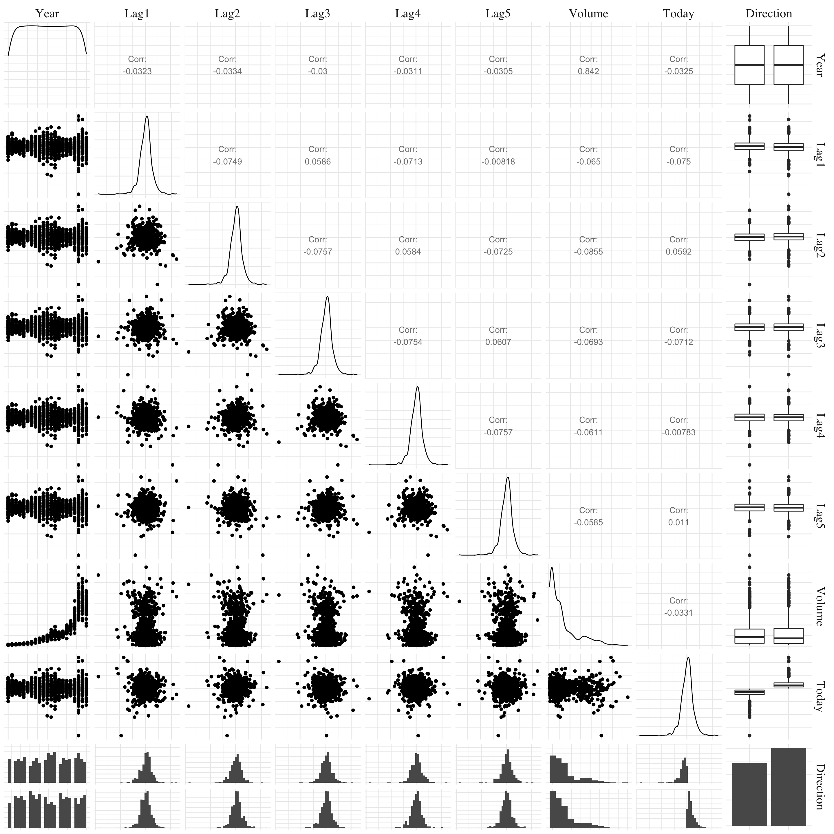
Figure 4.1: Pair plots.
We see a strong exponential pattern between the Year and Volume features.
- Question (b)
logit_model <- glm(Direction ~ Lag1 + Lag2 + Lag3 + Lag4 + Lag5 + Volume, data = weekly, family = 'binomial')
logit_model %>% summary() %>% print_summary_glm()- Formula: Direction ~ Lag1 + Lag2 + Lag3 + Lag4 + Lag5 + Volume
- Residuals
- Coefficients
- Null deviance: 1496.202 on 1088 degrees of freedom.
- Residual deviance: 1486.357 on 1082 degrees of freedom.
- AIC: 1500.357
| Name | NA_num | Unique | Range | Mean | Variance | Minimum | Q05 | Q10 | Q25 | Q50 | Q75 | Q90 | Q95 | Maximum |
|---|---|---|---|---|---|---|---|---|---|---|---|---|---|---|
| Residuals | 0 | 1089 | 3.15 | 0.04 | 1.36 | -1.69 | -1.35 | -1.32 | -1.26 | 0.99 | 1.08 | 1.14 | 1.17 | 1.46 |
| Variable | Estimate | Std. Error | z value | Pr(>|z|) |
|---|---|---|---|---|
| (Intercept) | 0.26686 | 0.08593 | 3.10561 | 0.0018988 |
| Lag1 | -0.04127 | 0.02641 | -1.56261 | 0.1181444 |
| Lag2 | 0.05844 | 0.02686 | 2.17538 | 0.0296014 |
| Lag3 | -0.01606 | 0.02666 | -0.60238 | 0.5469239 |
| Lag4 | -0.02779 | 0.02646 | -1.05014 | 0.2936533 |
| Lag5 | -0.01447 | 0.02638 | -0.54850 | 0.5833482 |
| Volume | -0.02274 | 0.03690 | -0.61633 | 0.5376748 |
Only one predictor appears to be statistically signicant in this model, the Lag2 feature.
- Question (c)
The function predict.glm gives the probability of the market going up between two weeks. This can be verified using the command contrasts(weekly$Direction).
logit_prob <- predict.glm(logit_model, type = 'response')
logit_pred <- if_else(logit_prob > .5, 'Up', 'Down')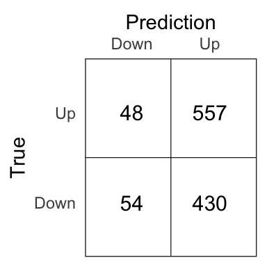
Figure 4.2: Confusion matrix for the complete logistic model.
The percentage of correct prediction of the movement of the market is 56.1%. However, if we set Up for avery prediction of the Direction variable, we will have a percentage of correct prediction of 55.6. So, the logistic regression improves very slightly the prediction accuracy. And, as we perform the prediction on the training set, it tends to overestimate the errors rate. The results on unseen data might (and should) be worse.
- Question (d)
logit_model <- glm(Direction ~ Lag2, data = train, family = 'binomial')
logit_prob <- predict(logit_model, newdata = test, type = 'response')
logit_pred <- if_else(logit_prob > .5, 'Up', 'Down')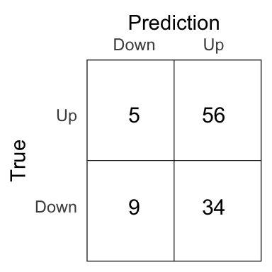
Figure 4.3: Confusion matrix for the logistic model on the test set.
The percentage of correct prediction of the movement of the market on the test set is 62.5% for the logistic model.
- Question (e)
lda_model <- lda(Direction ~ Lag2, data = train)
lda_prob <- predict(lda_model, test)$posterior[, 'Up']
lda_pred <- if_else(lda_prob > .5, 'Up', 'Down')
Figure 4.4: Confusion matrix for the LDA model on the test set.
The percentage of correct prediction of the movement of the market on the test set is 62.5% for the LDA model.
- Question (f)
qda_model <- qda(Direction ~ Lag2, data = train)
qda_prob <- predict(qda_model, test)$posterior[, 'Up']
qda_pred <- if_else(qda_prob > .5, 'Up', 'Down')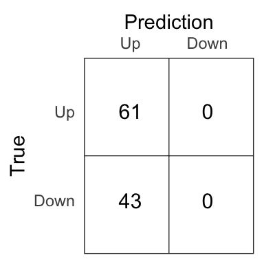
Figure 4.5: Confusion matrix for the QDA model on the test set.
The percentage of correct prediction of the movement of the market on the test set is 58.7% for the QDA model.
- Question (h)
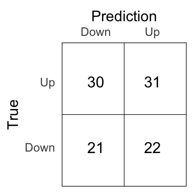
Figure 4.6: Confusion matrix for the \(K\)-NN model on the test set.
The percentage of correct prediction of the movement of the market on the test set is 50% for the \(K\)-NN model with \(K = 1\).
- Question (g)
Depending on what we want to emphasize, different methods provide the best results. If we are interested by the total accuracy (the number of good prediction), we should use the logistic model or the LDA model. But, if we want to just be good on the prediction of the Up, we must consider the QDA model (but the results on the Down prediction will be awful…). The \(K\)-NN does not provide good results, it really seems to overfit the training data.
- Question (i)
As none of the features (except Lag2) appear to be statistically significant in the logistic model, it seems unlikely that adding a combinaison of these features in the models will lead to better results. However, we can try to change the \(K\) in the \(K\)-NN algorithm to reduce the overfitting.
set.seed(42)
errors_rate <- c()
k <- seq(1, 20, by = 1)
for(i in k){
  knn_model <- knn(train[, 'Lag2'], test[, 'Lag2'], train$Direction, k = i)
  errors_rate <- c(errors_rate, round(100*mean(knn_model == test$Direction), 1))
}
df <- tibble(k = seq(1, 20, by = 1), errors_rate)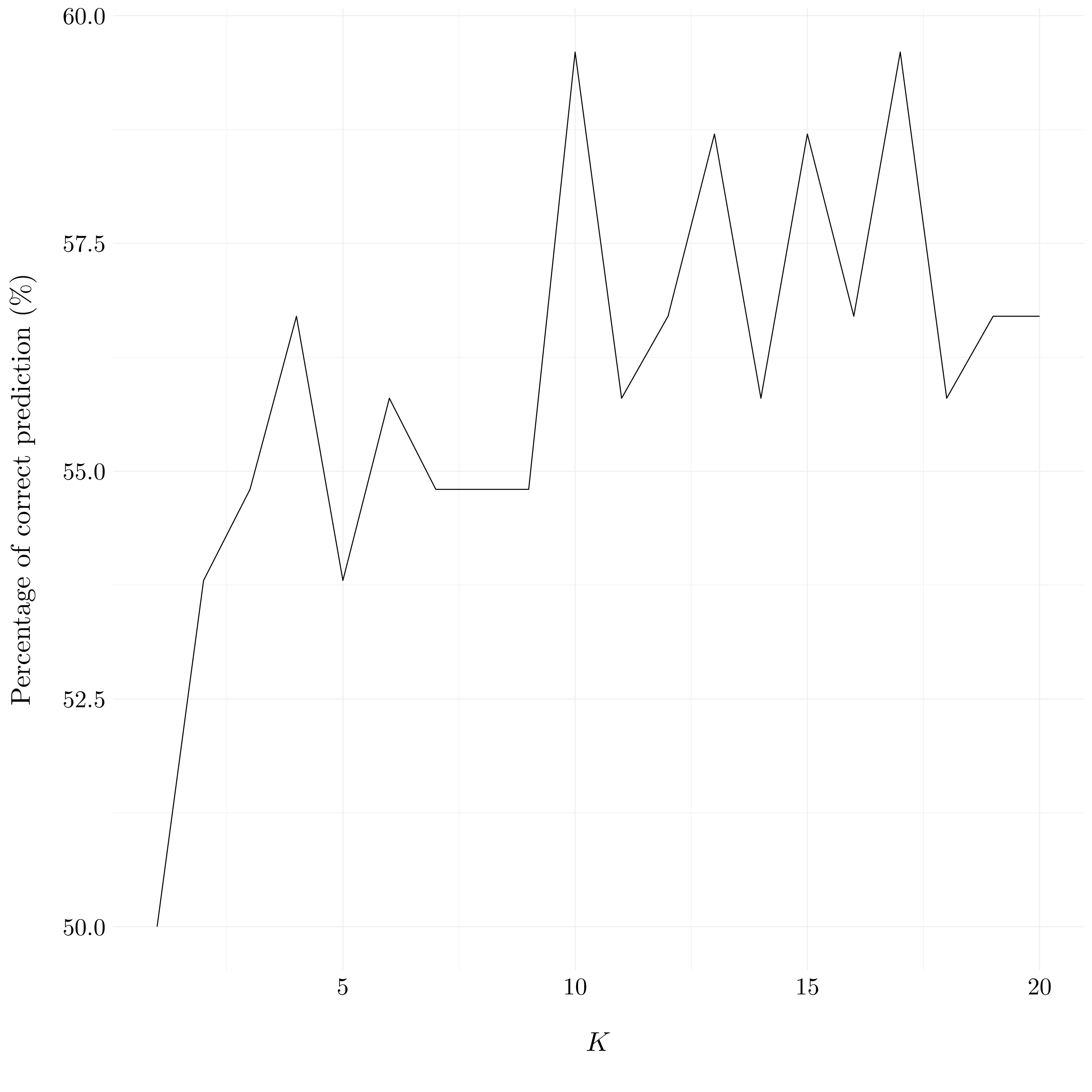
Figure 4.7: Evolution of percentage of correct predictions compared to \(K\).
For the \(K\)-NN model, we obtain the best results for \(K\) between 10 and 17. But, even here, the results are not as good as the ones of the logistic model and the LDA model.
4.2.2 Exercise 11.
- Question (a)
auto <- auto %>%
          mutate(mpg01 = if_else(mpg > median(mpg), 1, 0)) %>%
          mutate(mpg01 = as_factor(mpg01)) %>%
select(-c(mpg, name))- Question (b)
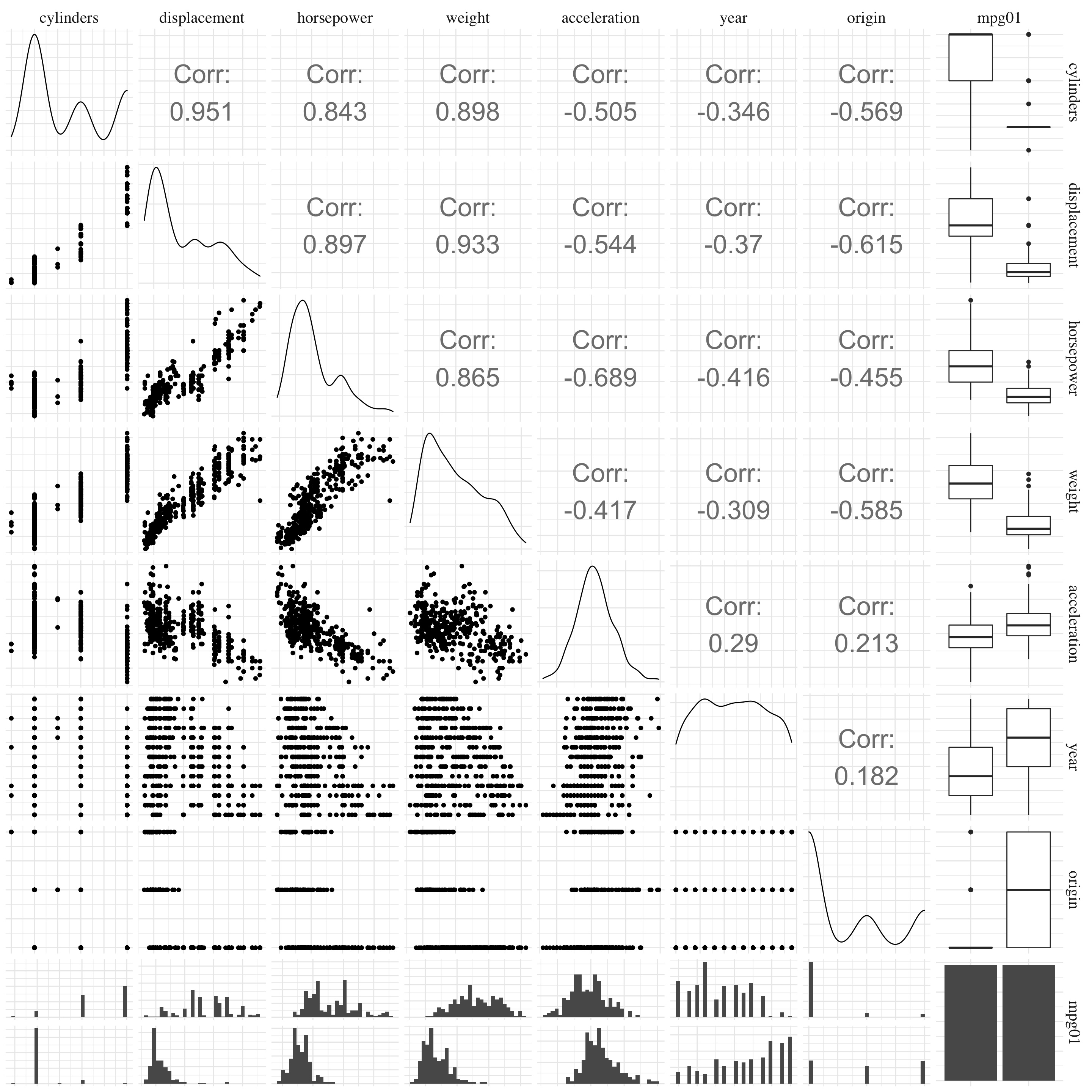
Figure 4.8: Pair plots.
Based on the pairs plot, four variables seem to be associated with the variable mpg01 and could be used to predict its value. These variables are cylinders, displacement, horsepower and weight. However, some of them appears to be particularly correlated (in particular, displacement with horsepower and weight). So, we have to be careful to not had redundant information in the model.
- Question (c)
set.seed(42)
idx <- auto$mpg01 %>% createDataPartition(p = 0.7, list = FALSE, times = 1)
train <- auto[idx[,1], ]
test <- auto[-idx[,1], ]- Question (d)
lda_model <- lda(mpg01 ~ cylinders + displacement + horsepower + weight, data = train)
lda_prob <- predict(lda_model, test)$posterior[, '1']
lda_pred <- if_else(lda_prob > .5, 1, 0)
Figure 4.9: Confusion matrix for the LDA model on the test set.
The test error of the LDA model is 0.09.
- Question (e)
qda_model <- qda(mpg01 ~ cylinders + displacement + horsepower + weight, data = train)
qda_prob <- predict(qda_model, test)$posterior[, '1']
qda_pred <- if_else(qda_prob > .5, 1, 0)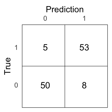
Figure 4.10: Confusion matrix for the QDA model on the test set.
The test error of the QDA model is 0.11.
- Question (f)
logit_model <- glm(mpg01 ~ cylinders + displacement + horsepower + weight, data = train, family = 'binomial')
logit_prob <- predict(logit_model, newdata = test, type = 'response')
logit_pred <- if_else(logit_prob > .5, 1, 0)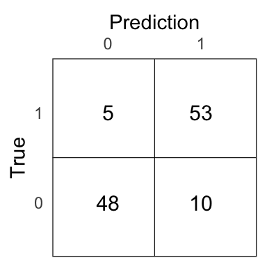
Figure 4.11: Confusion matrix for the logistic model on the test set.
The test error of the logistic model is 0.13.
- Question (g)
set.seed(42)
errors_rate <- c()
k <- seq(1, 100, by = 1)
for(i in k){
  knn_model <- knn(train[, c('cylinders', 'displacement', 'horsepower', 'weight')],
                   test[, c('cylinders', 'displacement', 'horsepower', 'weight')],
                   train$mpg01, k = i)
  errors_rate <- c(errors_rate, 1 - mean(knn_model == test$mpg01))
}
df <- tibble(k = seq(1, 100, by = 1), errors_rate)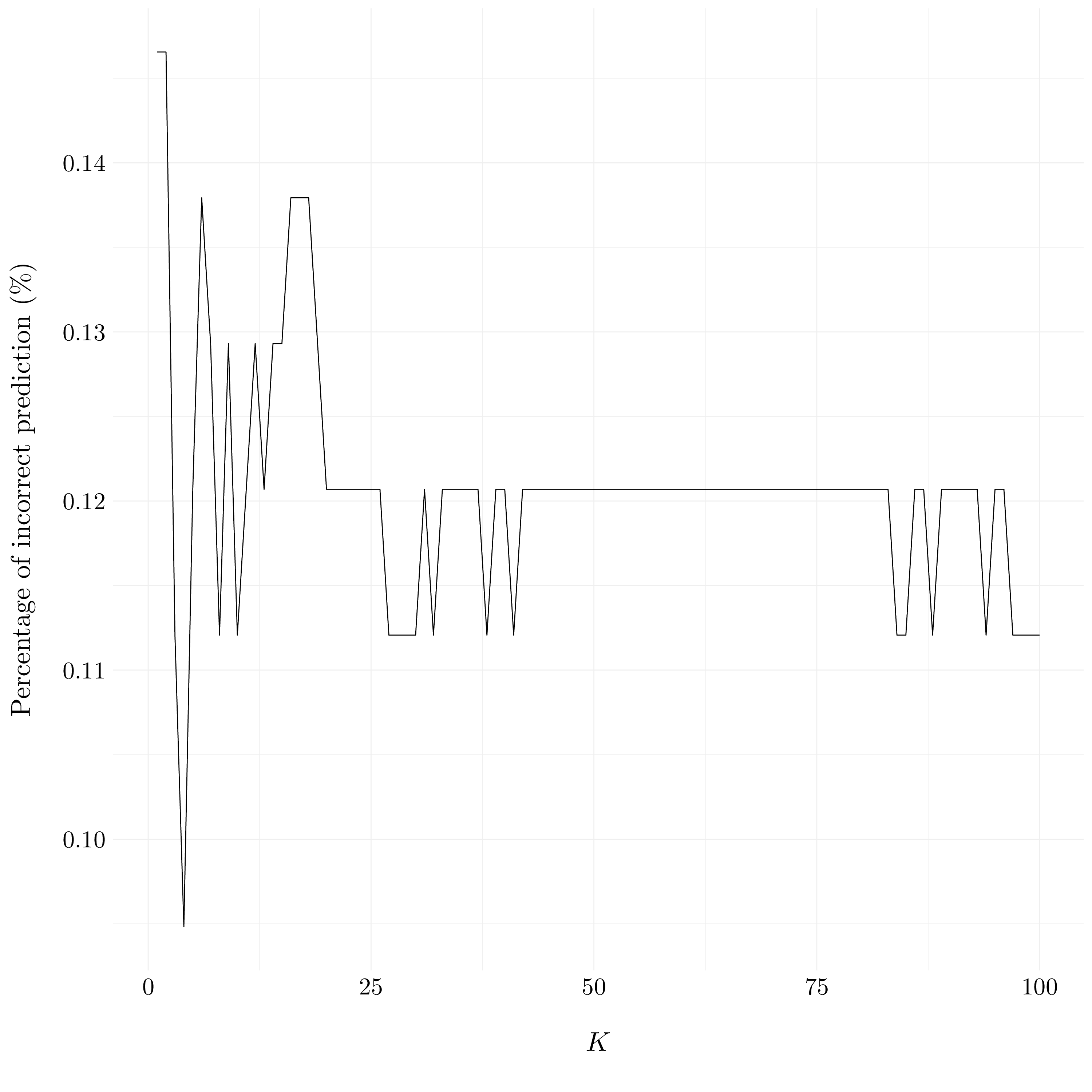
Figure 4.12: Evolution of percentage of incorrect predictions compared to \(K\).
The \(K\) which give the best results for the \(K\)-NN model is \(K = 3\).
4.2.3 Exercise 12.
Consider to look here.
4.2.4 Exercise 13.
boston <- boston %>%
            mutate(crim01 = if_else(crim > median(crim), 1, 0)) %>%
            mutate(crim01 = as_factor(crim01)) %>%
select(-c(crim))set.seed(42)
idx <- boston$crim01 %>% createDataPartition(p = 0.7, list = FALSE, times = 1)
train <- boston[idx[,1], ]
test <- boston[-idx[,1], ]lda_model <- lda(crim01 ~ ., data = train)
lda_prob <- predict(lda_model, test)$posterior[, '1']
lda_pred <- if_else(lda_prob > .5, 1, 0)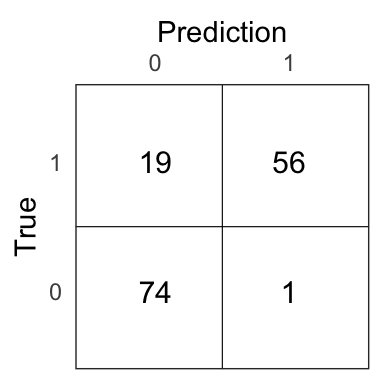
Figure 3.7: Confusion matrix for the LDA model on the test set.
The test error of the LDA model is 0.13.
qda_model <- qda(crim01 ~ ., data = train)
qda_prob <- predict(qda_model, test)$posterior[, '1']
qda_pred <- if_else(qda_prob > .5, 1, 0)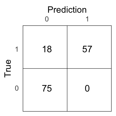
Figure 3.8: Confusion matrix for the QDA model on the test set.
The test error of the QDA model is 0.12.
logit_model <- glm(crim01 ~ ., data = train, family = 'binomial')
logit_prob <- predict(logit_model, newdata = test, type = 'response')
logit_pred <- if_else(logit_prob > .5, 1, 0)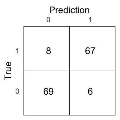
Figure 4.13: Confusion matrix for the logistic model on the test set.
The test error of the logistic model is 0.09.
set.seed(42)
errors_rate <- c()
k <- seq(1, 100, by = 1)
for(i in k){
  knn_model <- knn(select(train, -c('crim01')),
                   select(test, -c('crim01')),
                   train$crim01, k = i)
  errors_rate <- c(errors_rate, 1 - mean(knn_model == test$crim01))
}
df <- tibble(k = seq(1, 100, by = 1), errors_rate)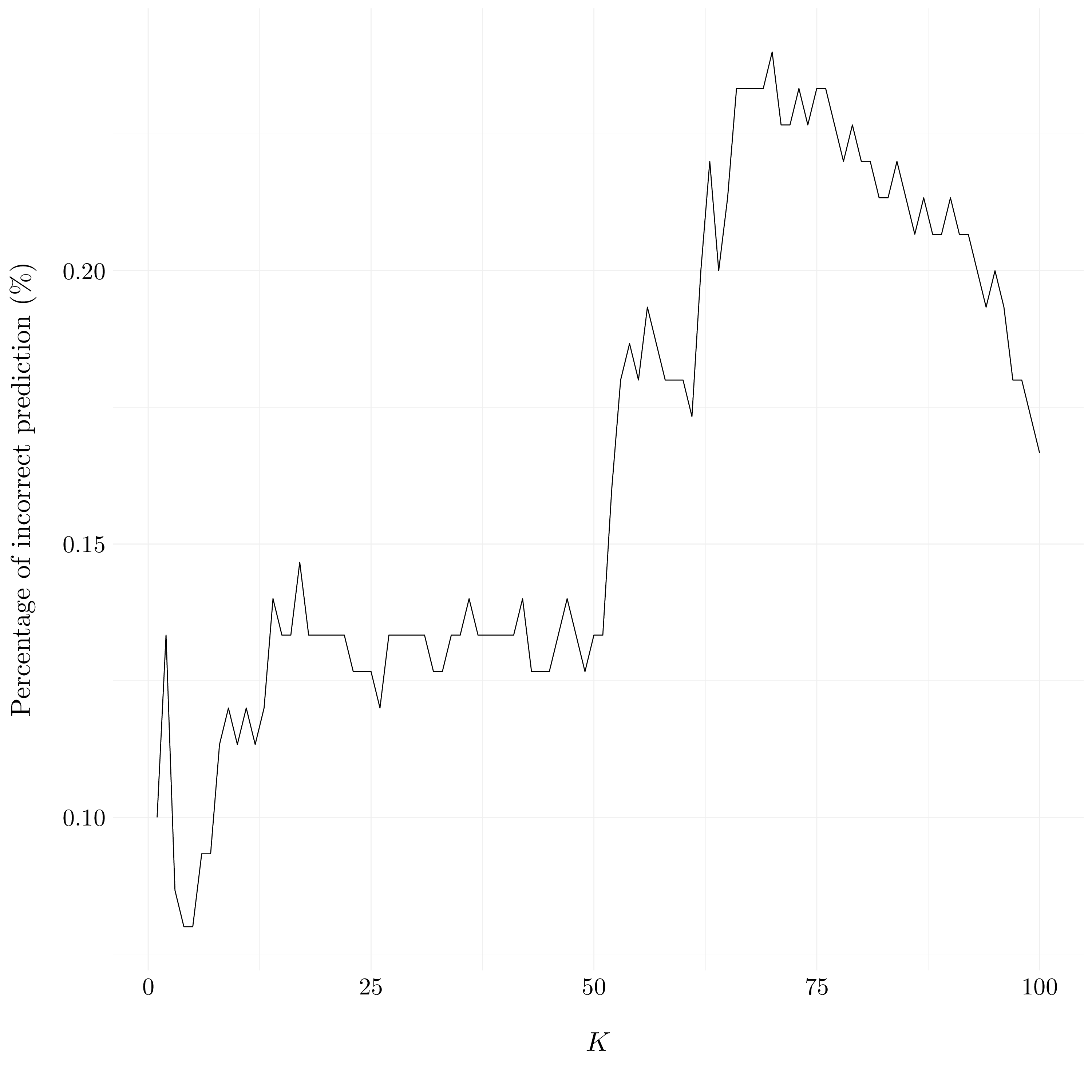
Figure 3.10: Evolution of percentage of incorrect predictions compared to \(K\).
The \(K\) which give the best results for the \(K\)-NN model is \(K = 4\) or \(K = 5\).