Chapter 7 Moving Beyond Linearity

7.1 Conceptual exercises

7.1.1 Exercise 1.

A cubic regression spline with one knot at \(\xi\) can be obtained using a basis of the form \(x, x^2, x^3, (x - \xi)_+^3\), where \((x - \xi)_+^3 = (x - \xi)^3\) if \(x > \xi\) and equals \(0\) otherwise. We will now show that a function of the form \[ f(x) = \beta_0 + \beta_1x + \beta_2x^2 + \beta_3x^3 + \beta_4(x - \xi)_+^3 \] is indeed a cubic regression spline, regardless of the values of \(\beta_0, \beta_1, \beta_2, \beta_3\) and \(\beta_4\).

Question (a)

Let’s define a function \[ f_1(x) = a_1 + b_1x + c_1x^2 + d_1x^3, \quad\text{for some real numbers}\quad a_1, b_1, c_1, d_1. \]

For all \(x \leq \xi\), \((x - \xi)_+^3 = 0\), and so we have \(f(x) = f_1(x)\) for all \(x \leq \xi\). And \(a_1 = \beta_0\), \(b_1 = \beta_1\), \(c_1 = \beta_2\) and \(d_1 = \beta_3\).

Question (b)

Let’s define a function \[ f_2(x) = a_2 + b_2x + c_2x^2 + d_2x^3, \quad\text{for some real numbers}\quad a_2, b_2, c_2, d_2. \]

For all \(x > \xi\), \((x - \xi)_+^3 = (x - \xi)^3 = x^3 - 3\xi x^2 + 3\xi^2 x - \xi^3\). Thus, we can rewrite \(f(x)\) as: \[ f(x) = (\beta_0 - \beta_4\xi^3) + (\beta_1 + 3\beta_4\xi^2)x + (\beta_2 - 3\beta_4\xi)x^2 + (\beta_3 + \beta_4)x^3.\]

Then, by identification, we found that \(a_2 = \beta_0 - \beta_4\xi^3\), \(b_2 = \beta_1 + 3\beta_4\xi^2\), \(c_2 = \beta_2 - 3\beta_4\xi\) and \(d_2 = \beta_3 + \beta_4\).

Question (c)

We have that: \[\begin{align*} f_2(\xi) &= (\beta_0 - \beta_4\xi^3) + (\beta_1 + 3\beta_4\xi^2)\xi + (\beta_2 - 3\beta_4\xi)\xi^2 + (\beta_3 + \beta_4)\xi^3 \\ &= \beta_0 + \beta_1\xi + \beta_2\xi^2 + \beta_3\xi^3 + (-\beta_4\xi^3 + 3\beta_4\xi^3 - 3\beta_4\xi^3 + \beta_4\xi^3) \\ &= f_1(\xi) \end{align*}\]

So, \(f(x)\) is continous at \(\xi\).

Question (d)

By taking the first derivatives: \[f_1^\prime(x) = \beta_1 + 2\beta_2x + 3\beta_3x^2 \quad\text{and}\quad f_2^\prime(x) = (\beta_1 + 3\beta_4\xi^2) + 2(\beta_2 - 3\beta_4\xi)x + 3(\beta_3 + \beta_4)x^2.\]

And so, \[\begin{align*} f_2^\prime(\xi) &= (\beta_1 + 3\beta_4\xi^2) + 2(\beta_2 - 3\beta_4\xi)\xi + 3(\beta_3 + \beta_4)\xi^2 \\ &= \beta_1 + 2\beta_2\xi + 3\beta_3\xi^2 + (3\beta_4\xi^2 - 6\beta_4\xi^2 + 3\beta_4\xi^2) \\ &= f_1^\prime(\xi) \end{align*}\]

So, \(f^\prime(x)\) is continuous at \(\xi\).

Question (e)

By taking the second derivatives: \[f_1^{\prime\prime}(x) = 2\beta_2 + 6\beta_3x \quad\text{and}\quad f_2^{\prime\prime}(x) = 2(\beta_2 - 3\beta_4\xi) + 6(\beta_3 + \beta_4)x.\]

And so, \[\begin{align*} f_2^{\prime\prime}(\xi) &= 2(\beta_2 - 3\beta_4\xi) + 6(\beta_3 + \beta_4)\xi \\ &= 2\beta_2 + 6\beta_3\xi - 6\beta_4\xi + 6\beta_4\xi \\ &= f_1^{\prime\prime}(\xi) \end{align*}\]

So, \(f^{\prime\prime}(x)\) is continuous at \(\xi\).

Therefore, \(f(x)\) is indeed a cubic sline.

7.1.2 Exercise 2.

Suppose that a curve \(\widehat{g}\) is computed to smoothly fit a set of \(n\) points using the following formula:

\[ \widehat{g} = \arg\min_g \left(\sum_{i=1}^n \left(y_i - g(x_i)\right)^2 + \lambda\int \left[g^{(m)}(x)\right]^2dx\right),\] where \(g^{(m)}\) represents the \(m\)th derivatives of \(g\) (and \(g^{(0)} = g\)).

Question (a)

When \(\lambda = \infty\) and \(m = 0\), \(\widehat{g}\) will be perfectly smooth and so \(\int \left[g^{(0)}(x)\right]^2dx\) should be very close to \(0\). Thus, we find that \(\widehat{g}\) will be equal to \(0\).

Question (b)

When \(\lambda = \infty\) and \(m = 1\), \(\widehat{g}\) will be perfectly smooth and so \(\int \left[g^{(1)}(x)\right]^2dx\) should be very close to \(0\). Thus, we find that \(\widehat{g}\) will be a constant function (of the form \(\widehat{g}(x) = k\)).

Question (c)

When \(\lambda = \infty\) and \(m = 2\), \(\widehat{g}\) will be perfectly smooth and so \(\int \left[g^{(2)}(x)\right]^2dx\) should be very close to \(0\). Thus, we find that \(\widehat{g}\) will be a linear function (of the form \(\widehat{g}(x) = ax + b\)).

Question (d)

When \(\lambda = \infty\) and \(m = 3\), \(\widehat{g}\) will be perfectly smooth and so \(\int \left[g^{(3)}(x)\right]^2dx\) should be very close to \(0\). Thus, we find that \(\widehat{g}\) will be equal a quadratic function (of the form \(\widehat{g}(x) = ax^2 + bx + c\)).

Question (e)

When \(\lambda = 0\) and \(m = 3\), we do not put any constraints on \(g(x_i)\), then \(\widehat{g}\) will be such that it interpolates all of the \(y_i\).

7.1.3 Exercise 3.

Suppose we fit a curve with basis functions: \[\begin{align*} b_1(X) &= X \\ b_2(X) &= (X - 1)^2\mathbf{1}(X \geq 1) \end{align*}\]

We fit the linear regression model \[ Y = \beta_0 + \beta_1b_1(X) + \beta_2b_2(X) + \epsilon,\] and obtain coefficient estimates \(\widehat{\beta}_0 = 1, \widehat{\beta}_1 = 1\) and \(\widehat{\beta}_2 = -2\).

X <- seq(-2, 2, 0.1)
Y <- 1 + X - 2 * (X - 1)**2 * (X > 1)

Figure 7.1: Sketch of the estimated curve between \(X = -2\) and \(X = 2\)

7.1.4 Exercise 4.

Suppose we fit a curve with basis functions \[\begin{align*} b_1(X) &= \mathbf{1}(0 \leq X \leq 2) - (X - 1)\mathbf{1}(1 \leq 2) \\ b_2(X) &= (X - 3)\mathbf{1}(3 \leq X \leq 4) + \mathbf{1}(4 < X \leq 5) \end{align*}\]

b1 <- function(x) (x >= 0 & x <= 2) - (x - 1) * (x >= 1 & x <= 2)
b2 <- function(x) (x - 3) * (x >= 3 & x <= 4) + (x > 4 & x <= 5)
X <- seq(-5, 5, 0.1)
Y <- 1 + b1(X) + 3 * b2(X)

Figure 7.2: Sketch of the estimated curve between \(X = -5\) and \(X = 5\)

7.1.5 Exercise 5.

Consider two curves, \(\widehat{g}_1\) and \(\widehat{g}_2\), defined by

\[\widehat{g}_1 = \arg\min_g \left(\sum_{i=1}^n \left(y_i - g(x_i)\right)^2 + \lambda\int \left[g^{(3)}(x)\right]^2dx\right),\]

\[\widehat{g}_2 = \arg\min_g \left(\sum_{i=1}^n \left(y_i - g(x_i)\right)^2 + \lambda\int \left[g^{(4)}(x)\right]^2dx\right)\]

where \(g^{(m)}\) represents the \(m\)th derivative of \(g\).

Question (a)

As \(\lambda \rightarrow \infty\), \(\widehat{g}_2\) will have the smaller training RSS because \(\widehat{g}_2\) should be more flexible than \(\widehat{g}_1\) (less constraints), so it should better fit the training data and lead to a smaller training RSS.

Question (b)

As \(\lambda \rightarrow \infty\), we can not say which function will have the smaller test RSS because it depends on the true underlying function \(g\). If the true function \(g\) is a polynomial function with degree at most 2, then \(\widehat{g}_1\) will likely have the smaller test RSS (because \(\widehat{g}_2\) will overfit). Once, the true function is a polynomial function with degree larger than 3, it should be the other way round.

Question (c)

For \(\lambda = 0\), \(\widehat{g}_1\) and \(\widehat{g}_2\) become the same function, so they will have the same training and test RSS.

7.2 Applied exercises

7.2.1 Exercise 6.

wage <- as_tibble(Wage)
X <- wage$age; Y <- wage$wage

Question (a)

We aim to predict wage using age with polynomial regression of degree \(d\). The degree will be chosen by cross-validation.

fits <- list()
cv_error <- vector(length = 10)

set.seed(42)
for(d in 1:10){
  fits[d] <- list(lm(wage ~ poly(age, d), data = wage))
  fit <- glm(wage ~ poly(age, d), data = wage)
  cv_error[d] <- cv.glm(wage, fit, K = 10)$delta[2]
}

Figure 7.3: Cross-validation errors according to the considered degree.

So, according to cross-validation, the best degree to fit the wage is 9.

Now, we will compare the chosen degree with the one obtained by hypothesis testing using ANOVA. ANOVA tests the null hypothesis that a model \(\mathcal{M}_1\) is sufficient to explain the data against the alternative hypothesis that a more complex model \(\mathcal{M}_2\) is required. Careful, \(\mathcal{M}_1\) and \(\mathcal{M}_2\) must be nested.

do.call(anova, fits)

## Analysis of Variance Table
## 
## Model  1: wage ~ poly(age, d)
## Model  2: wage ~ poly(age, d)
## Model  3: wage ~ poly(age, d)
## Model  4: wage ~ poly(age, d)
## Model  5: wage ~ poly(age, d)
## Model  6: wage ~ poly(age, d)
## Model  7: wage ~ poly(age, d)
## Model  8: wage ~ poly(age, d)
## Model  9: wage ~ poly(age, d)
## Model 10: wage ~ poly(age, d)
##    Res.Df     RSS Df Sum of Sq        F    Pr(>F)    
## 1    2998 5022216                                    
## 2    2997 4793430  1    228786 143.7638 < 2.2e-16 ***
## 3    2996 4777674  1     15756   9.9005  0.001669 ** 
## 4    2995 4771604  1      6070   3.8143  0.050909 .  
## 5    2994 4770322  1      1283   0.8059  0.369398    
## 6    2993 4766389  1      3932   2.4709  0.116074    
## 7    2992 4763834  1      2555   1.6057  0.205199    
## 8    2991 4763707  1       127   0.0796  0.777865    
## 9    2990 4756703  1      7004   4.4014  0.035994 *  
## 10   2989 4756701  1         3   0.0017  0.967529    
## ---
## Signif. codes:  0 '***' 0.001 '**' 0.01 '*' 0.05 '.' 0.1 ' ' 1

Then, the results are the same than the ones from the book (p. 270). The p-value comparing the linear model to the quadratic model is essentially zero (\(< 10^{-15}\)), indicating that a linear fit is not sufficient. Similarly the p-value comparing the quadratic model to the cubic model is very low, so the quadratic fit is also insufficient. The p-value comparing the cubic and the quadric models is approximately \(5\%\) while the degree-5 polynomial seems unnecessary because its high p-value. Hence, either a cubic or a quartic polynomial appear to provide a reasonable fit to the data, but lower- or higher-order models are not justified. These results are quite similar to the cross-validation ones. Even if the cubic or quartic polynomial have not the smallest CV errors, they are quite close to the best.

Finally, let’s fit the data with a degree-4 polynomial and plot it.

fit_final <- glm(wage ~ poly(age, 4), data = wage)
pred <- predict(fit_final, newdata = list(age = X), se.fit = TRUE)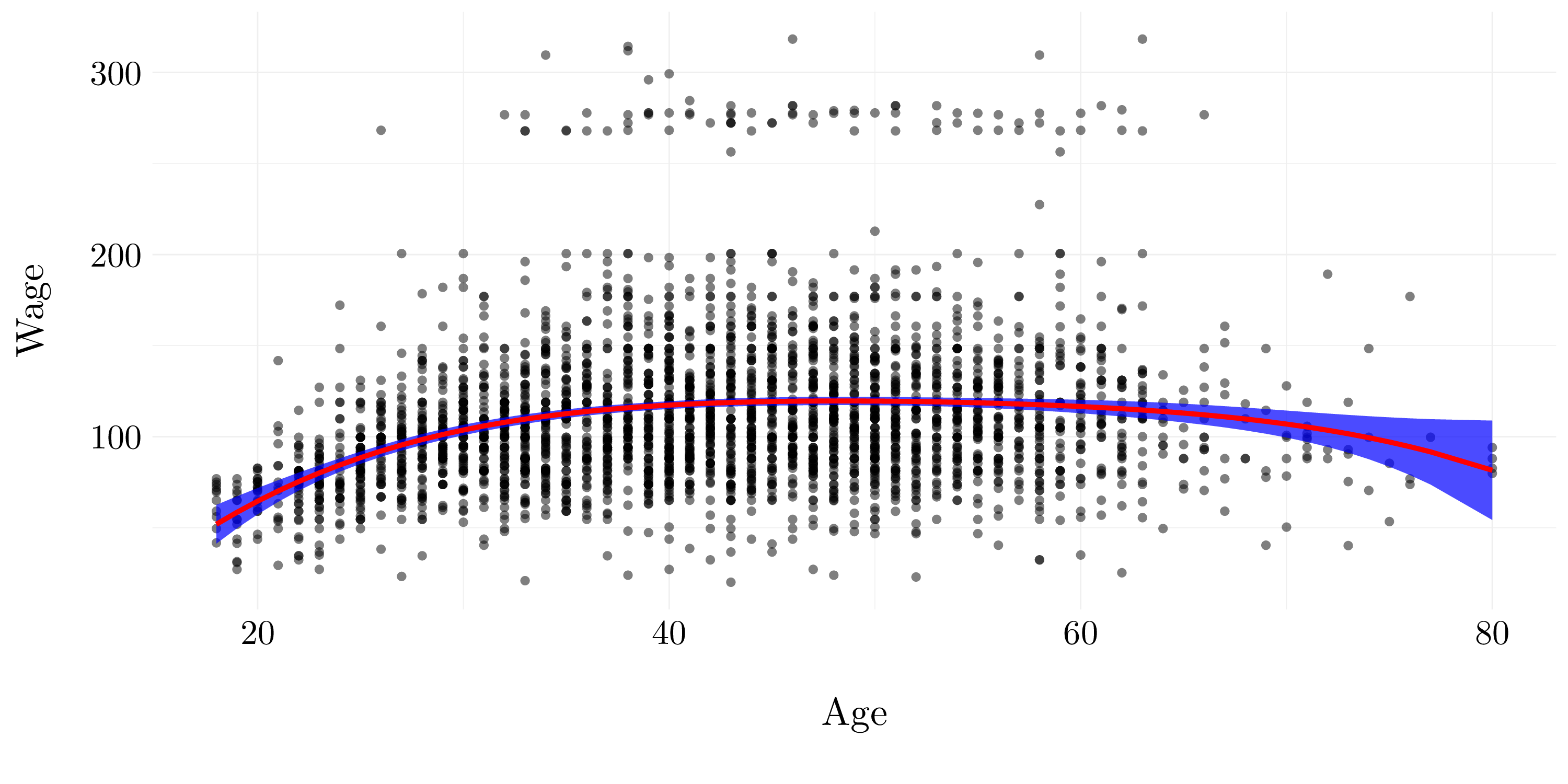

Figure 7.4: Quadric polynomial model.

Question (b)

Let’s fit a step function to predict wage using age, and perform cross-validation to choose the optimal number of cuts.

cv_error <- vector()

set.seed(42)
for(d in 2:15){
  wage$age_cut <- cut(wage$age, d)
  fit <- glm(wage ~ age_cut, data = wage)
  cv_error[d-1] <- cv.glm(wage, fit, K = 10)$delta[2]
}

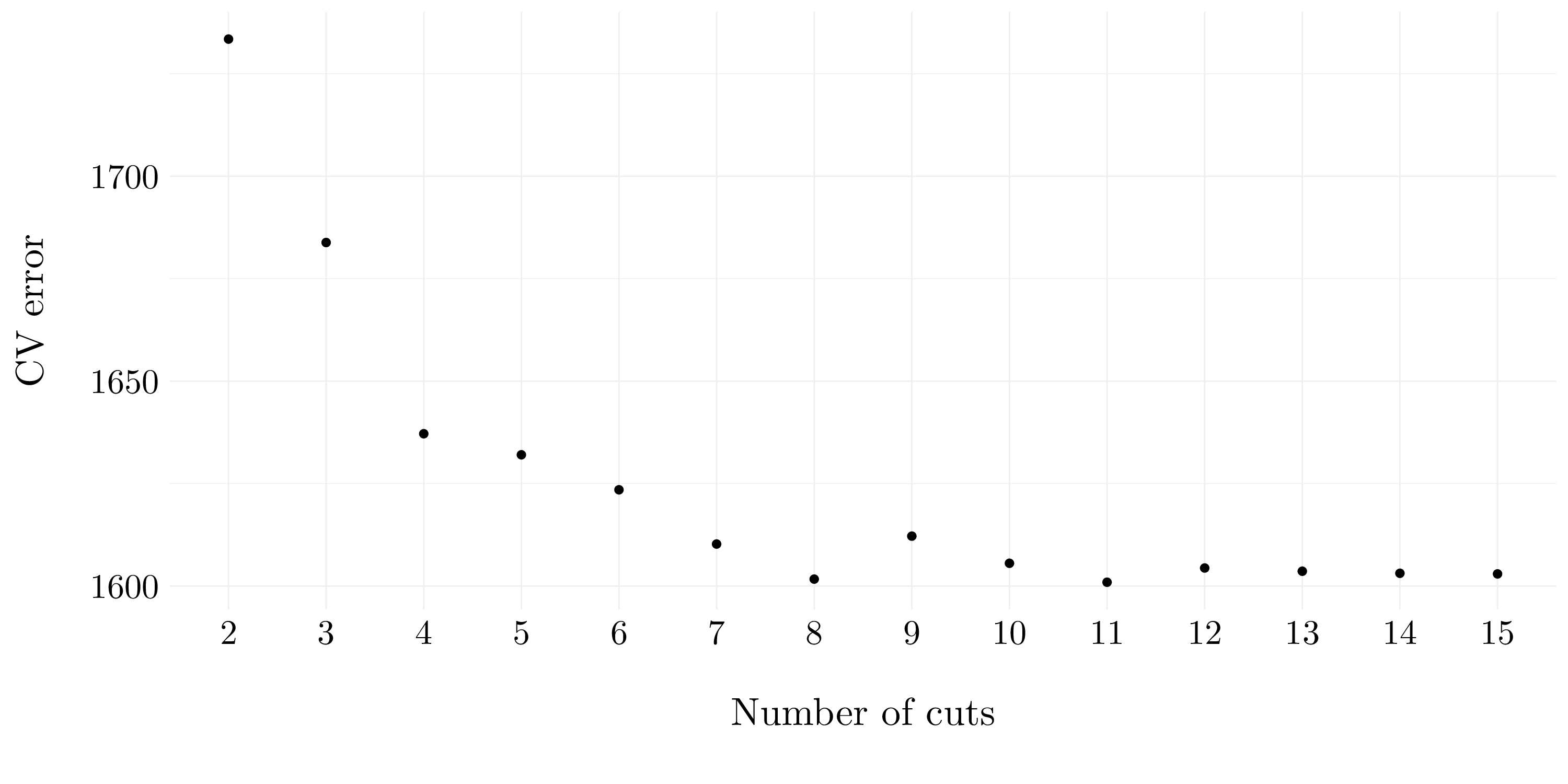
Figure 7.5: Cross-validation errors according to the considered number of cuts.

So, according to cross-validation, the best number of cuts to fit the wage is 11.

Finally, let’s fit the data with 11 cuts for the age and plot it.

wage$age_cut <- cut(wage$age, which.min(cv_error) + 1)
fit_final <- glm(wage ~ age_cut, data = wage)
pred <- predict(fit_final, newdata = list(age_cut = cut(X, which.min(cv_error) + 1)), se.fit = TRUE)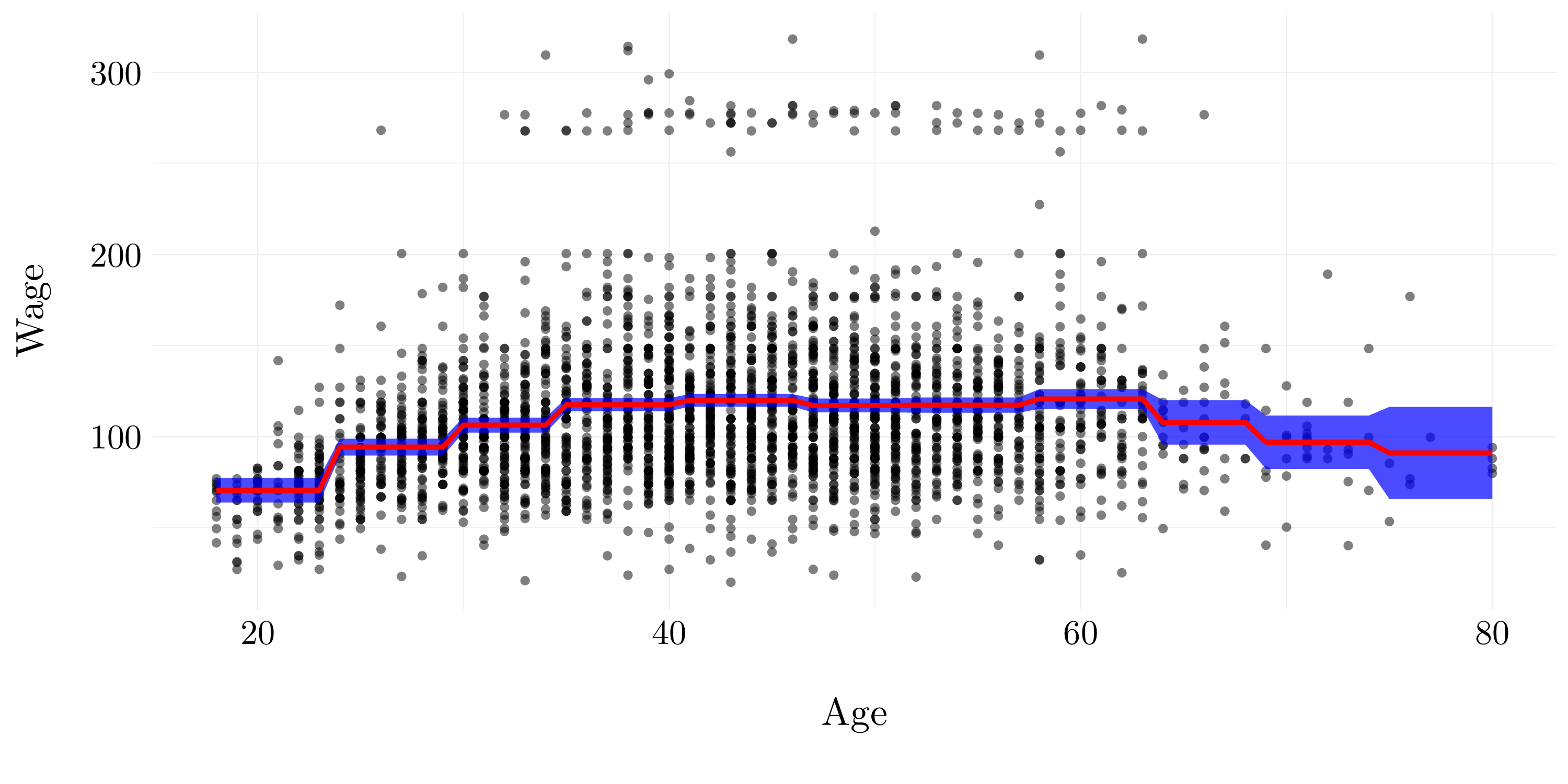

Figure 7.6: Step model.

7.2.2 Exercise 7.

wage <- as_tibble(Wage)
X <- wage$age; Y <- wage$wage

Let’s explore relationships between the different variables in the wage dataset. For that, first, we are going to compute the correlation between the features and the ouput wage.

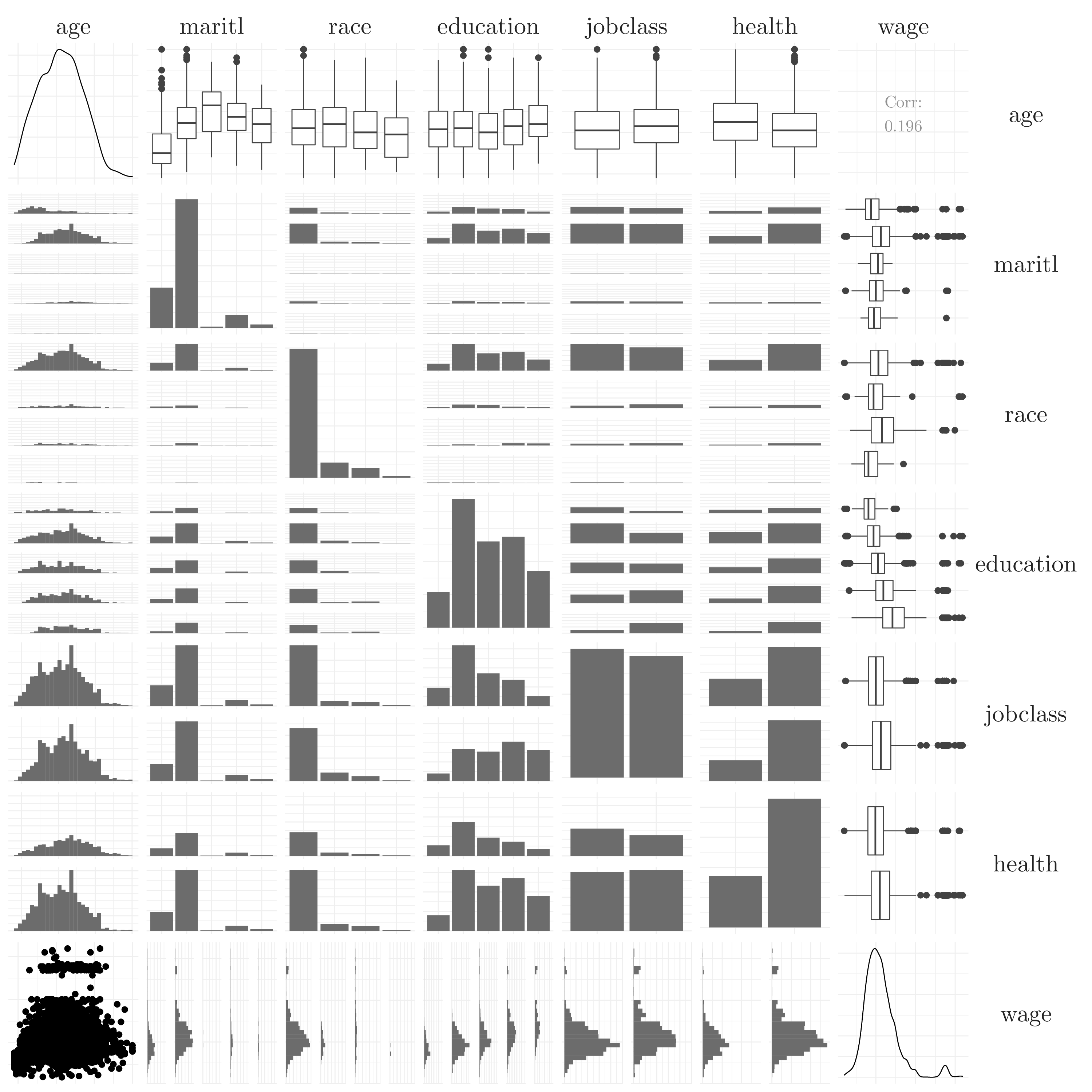
Figure 7.7: Correlation plot.

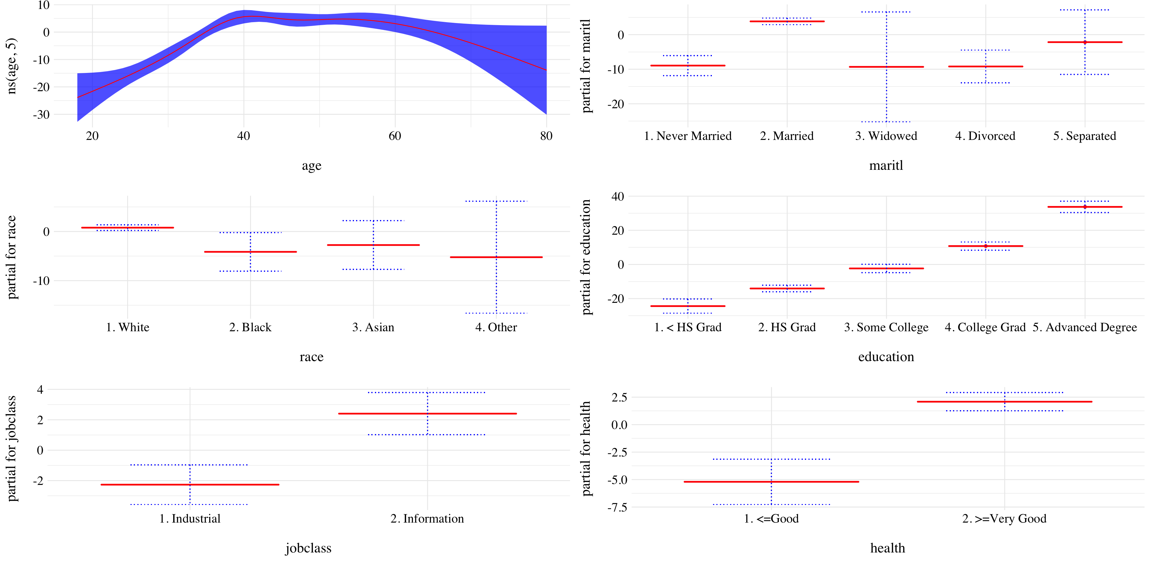
fit_gam <- gam(wage ~ ns(age, 5) + maritl + race + education + jobclass + health, data = wage)

Figure 7.8: Results of the GAM.

The results are pretty intuitive. With other variables being fixed, wage tends to be highest for intermediate values of age, and lowest for the very young and the very old. With other variables being fixed, wage tends to increase with education. The more educated a person is, the higher their salary, on average. Same, people with very good health have a higher wage than the one with less good health. Moreover, information jobs are more paid than industrial ones. Finally, white and married people seems to earn more money.

7.2.3 Exercise 8.

auto <- as_tibble(Auto)

Let’s explore relationship between the different variables in the wage dataset. For that, first, we are going to compute the correlation between the variables.

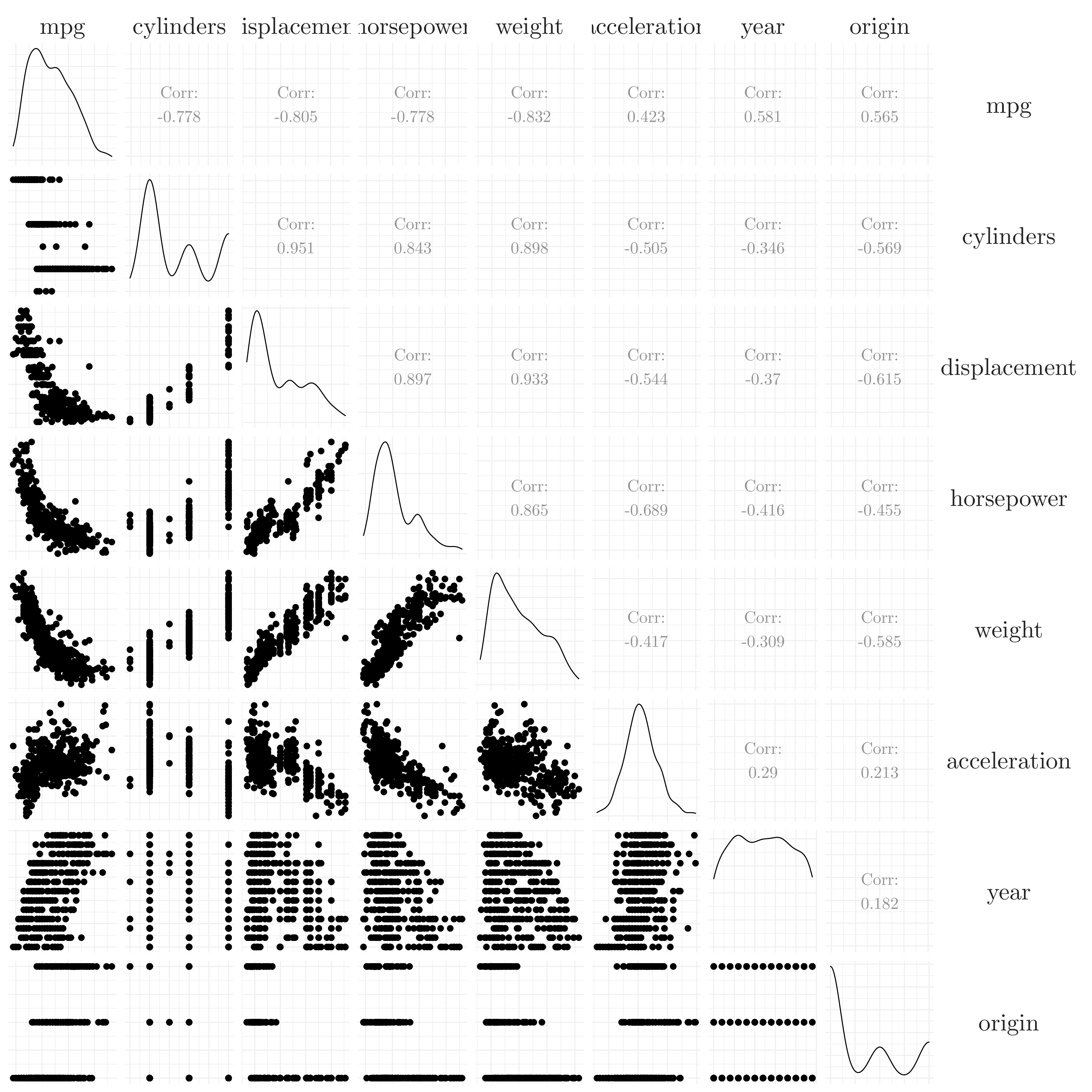
Figure 7.9: Correlation plot.

We are going to use the mpg variable as a output. Most of the other variables seem to have a non-linear relationship with the variable mpg. Let’s use the displacement in order to predict the mpg variable.

fits <- list()
cv_error <- vector(length = 10)

set.seed(42)
for(d in 1:10){
  fits[d] <- list(lm(mpg ~ bs(displacement, df = d), data = auto))
  fit <- glm(mpg ~ bs(displacement, df = d), data = auto)
  cv_error[d] <- cv.glm(auto, fit, K = 10)$delta[2]
}

Figure 7.10: Cross-validation errors according to the degree of freedom of the B-splines.

fit_final <- glm(mpg ~ bs(displacement, df = 7), data = auto)
pred <- predict(fit_final, newdata = list(displacement = auto$displacement), se.fit = TRUE)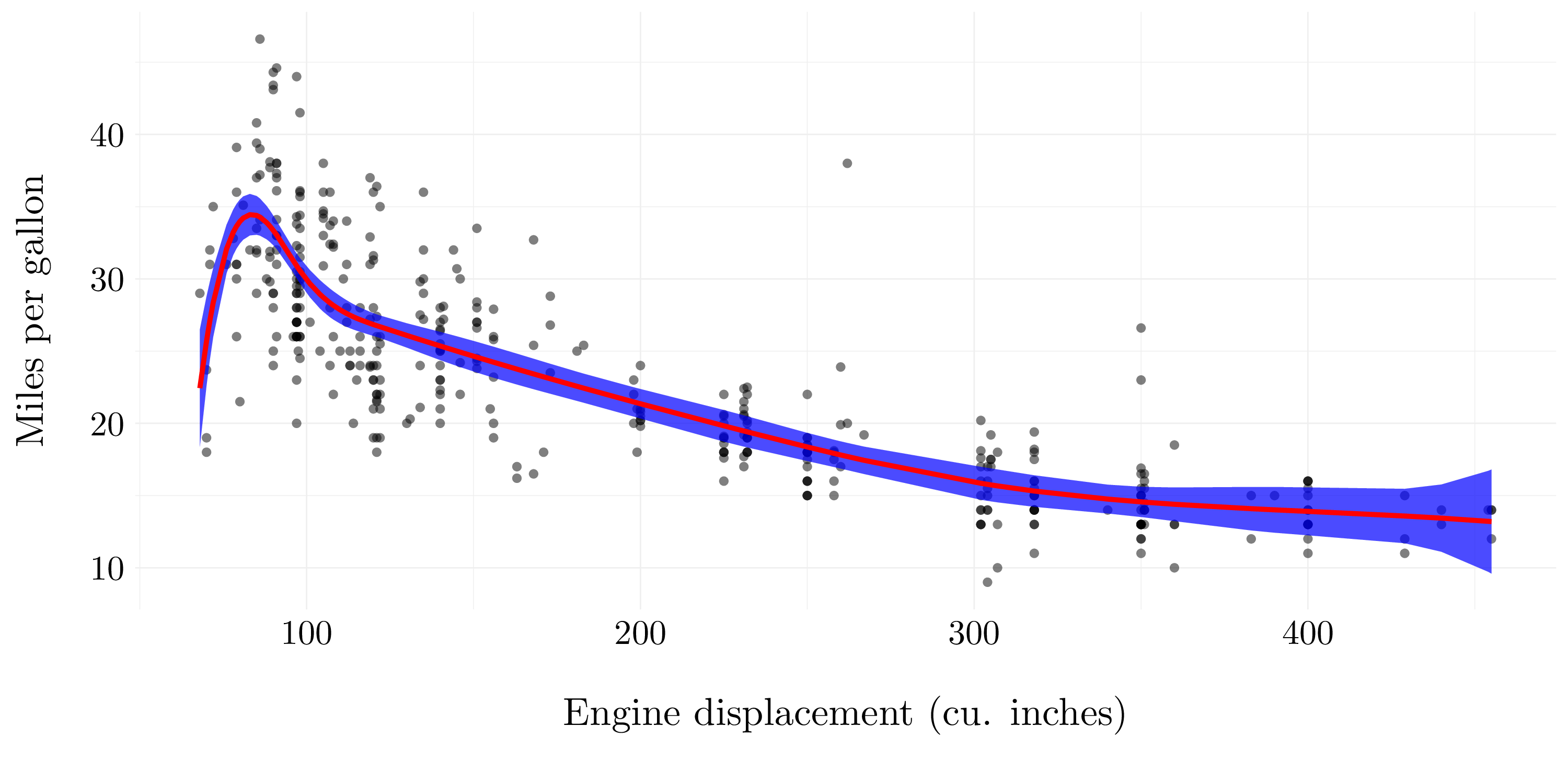

Figure 7.11: B-spline model with 7 degree of freedom.

7.2.4 Exercise 9.

boston <- as_tibble(Boston)

We uses the variables dis (the weighted mean of distances to five Boston employment centers) and nox (nitrogen oxides concentration in parts per 10 million) from the Boston data. We will treat dis as the predictor and nox as the response.

Question (a)

model_poly <- lm(nox ~ poly(dis, 3), data = boston)

Results of the linear model on the boston dataset.

Formula: nox ~ poly(dis, 3)
Residuals

Name	NA_num	Unique	Range	Mean	Variance	Minimum	Q05	Q10	Q25	Q50	Q75	Q90	Q95	Maximum
Residuals	0	418	0.32	0	0	-0.12	-0.08	-0.07	-0.04	-0.01	0.02	0.09	0.13	0.19

Coefficients

Variable	Estimate	Std. Error	t value	Pr(>\|t\|)
(Intercept)	0.55470	0.00276	201.02089	< 2.22e-16
poly(dis, 3)1	-2.00310	0.06207	-32.27107	< 2.22e-16
poly(dis, 3)2	0.85633	0.06207	13.79599	< 2.22e-16
poly(dis, 3)3	-0.31805	0.06207	-5.12396	4.275e-07

Residual standard error: 0.062 on 502 degrees of freedom.
Multiple \(R^2\): 0.715.
Adjusted \(R^2\): 0.713.
F-statistic: 419.335 on 3 and 502, p-value: <2e-16.

pred <- predict(model_poly, newdata = list(dis = boston$dis), se.fit = TRUE)

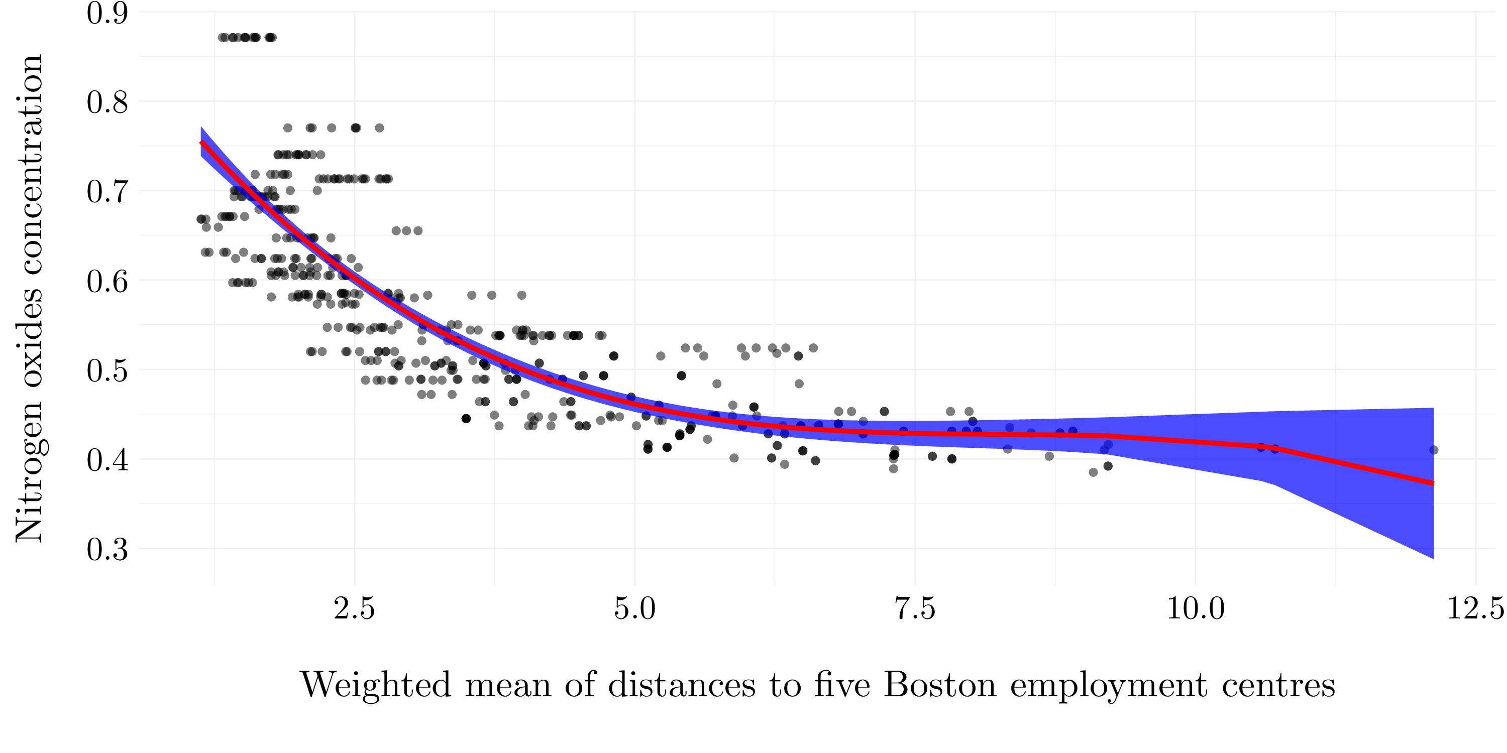
Figure 7.12: Cubic polynomial regression model

Question (b)

res <- list()

set.seed(42)
for(d in 2:10){
  fit <- lm(nox ~ poly(dis, d), data = boston)
  res[[d-1]] <- list(d = d, pred = predict(fit, newdata = list(dis = boston$dis), se.fit = TRUE))
}

ggfit <- function(d, pred){
  ggplot(aes(x = dis, y = nox), data = boston) +
    geom_point(alpha = 0.5) +
    geom_ribbon(aes(ymin = pred$fit - 2*pred$se.fit, ymax = pred$fit + 2*pred$se.fit), alpha = 0.7, fill = 'blue') +
    geom_line(aes(x = boston$dis, y = pred$fit), col = 'red', lwd = 2) +
    ggtitle(paste('Degree: ', d, '(RSS = ', round(sum((boston$nox - pred$fit)**2), 2), ')')) +
    xlab('Weighted mean of distances to five Boston employment centres') +
    ylab('Nitrogen oxides concentration') +
    theme_custom()
}

plot_list <- res %>% map(~ ggfit(.x$d, .x$pred))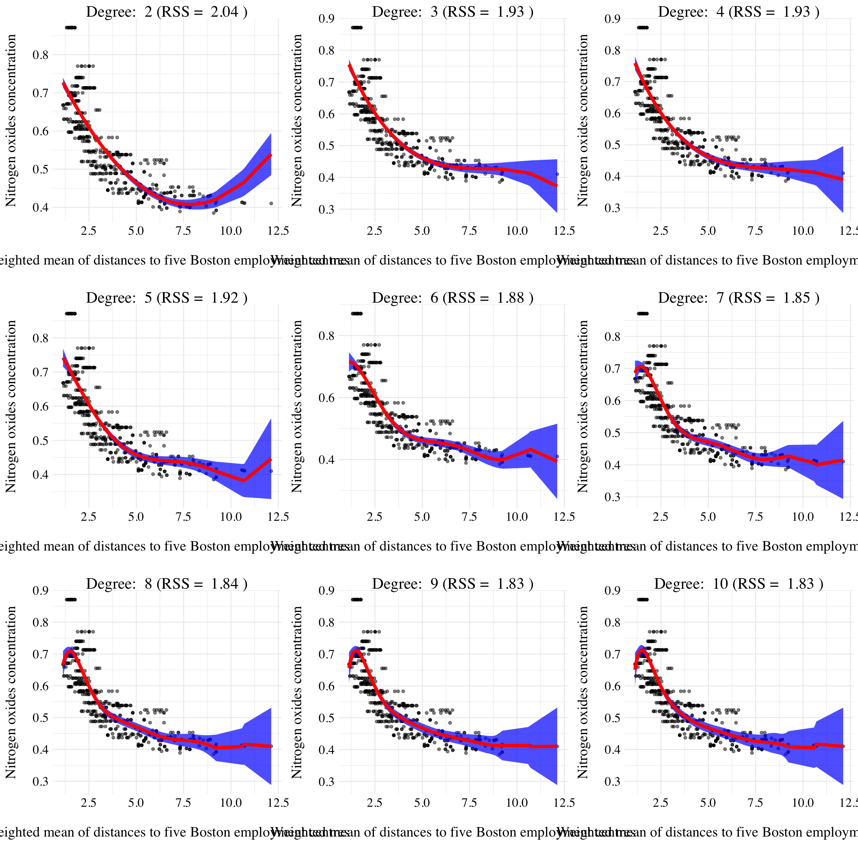

Figure 7.13: Results of polynomial fits.

Question (c)

fits <- list()
cv_error <- vector(length = 10)

set.seed(42)
for(d in 1:10){
  fits[d] <- list(lm(nox ~ poly(dis, d), data = boston))
  fit <- glm(nox ~ poly(dis, d), data = boston)
  cv_error[d] <- cv.glm(boston, fit, K = 10)$delta[2]
}

Figure 7.14: Cross-validation errors according to the considered degree.

Question (d)

We fit a regression spline using four degrees of freedom to predict nox using dis. We choose the knots to be the quantile of dis.

model_spline <- lm(nox ~ bs(dis, df = 4), data = boston)

Results of the linear model on the boston dataset.

Formula: nox ~ bs(dis, df = 4)
Residuals

Name	NA_num	Unique	Range	Mean	Variance	Minimum	Q05	Q10	Q25	Q50	Q75	Q90	Q95	Maximum
Residuals	0	420	0.32	0	0	-0.12	-0.08	-0.07	-0.04	-0.01	0.02	0.09	0.13	0.19

Coefficients

Variable	Estimate	Std. Error	t value	Pr(>\|t\|)
(Intercept)	0.73447	0.01460	50.30552	< 2.22e-16
bs(dis, df = 4)1	-0.05810	0.02186	-2.65782	0.008116
bs(dis, df = 4)2	-0.46356	0.02366	-19.59614	< 2.22e-16
bs(dis, df = 4)3	-0.19979	0.04311	-4.63395	4.5805e-06
bs(dis, df = 4)4	-0.38881	0.04551	-8.54394	< 2.22e-16

Residual standard error: 0.062 on 501 degrees of freedom.
Multiple \(R^2\): 0.716.
Adjusted \(R^2\): 0.714.
F-statistic: 316.463 on 4 and 501, p-value: <2e-16.

pred <- predict(model_spline, newdata = list(dis = boston$dis), se.fit = TRUE)

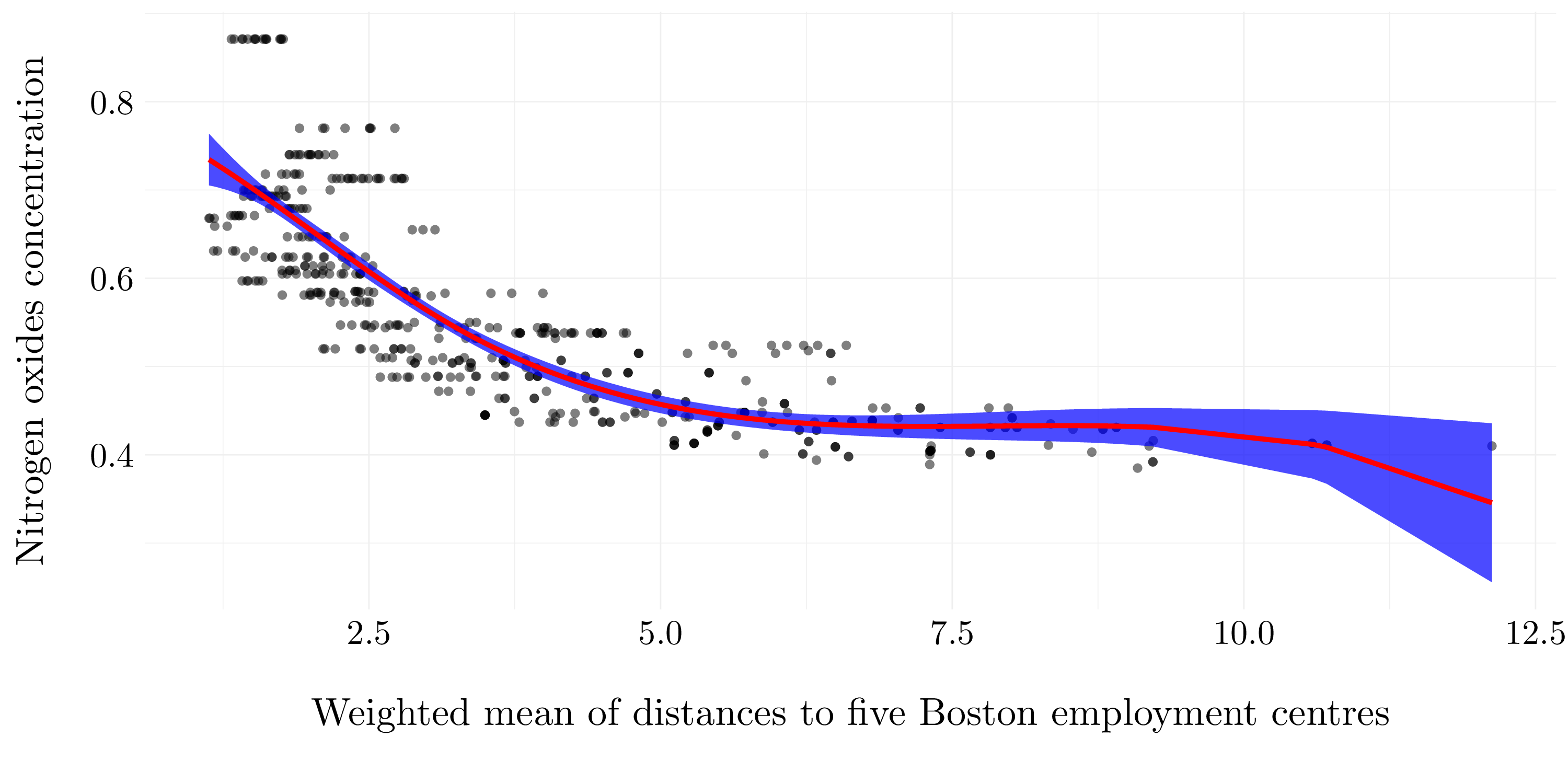
Figure 7.15: Four degrees of freedom spline regression model

Question (e)

res <- list()

set.seed(42)
for(d in 2:10){
  fit <- lm(nox ~ bs(dis, df = d), data = boston)
  res[[d-1]] <- list(d = d, pred = predict(fit, newdata = list(dis = boston$dis), se.fit = TRUE))
}

plot_list <- res %>% map(~ ggfit(.x$d, .x$pred))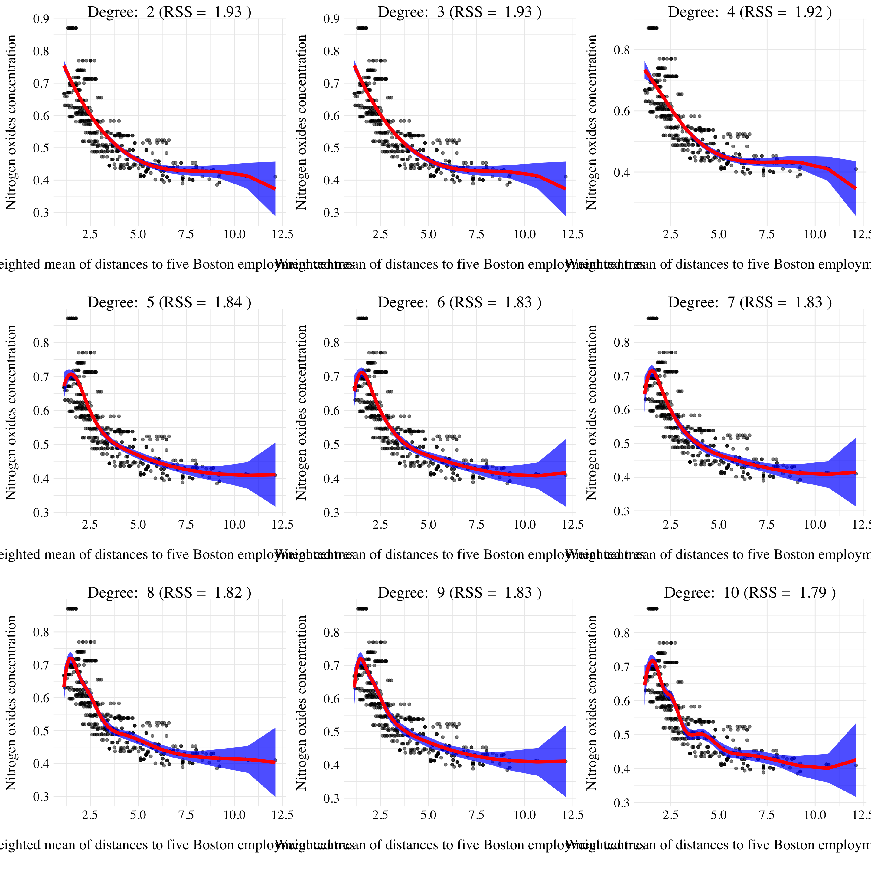

Figure 7.16: Results of splines fits.

Question (f)

fits <- list()
cv_error <- vector(length = 10)

set.seed(42)
for(d in 1:10){
  fits[d] <- list(lm(nox ~ bs(dis, df = d), data = boston))
  fit <- glm(nox ~ bs(dis, df = d), data = boston)
  cv_error[d] <- cv.glm(boston, fit, K = 10)$delta[2]
}

Figure 7.17: Cross-validation errors according to the considered degree.

7.2.5 Exercise 10.

We are going to analize the College data set.

college <- as_tibble(College)

Question (a)

Let’s split the data set into training set and test set.

idx <- sample(1:nrow(college), size = round(0.5 * nrow(college)))
train <- college %>% slice(idx)
test <- college %>% slice(-idx)

reg_subset <- regsubsets(Outstate ~ ., data = train, nvmax = 10, method = 'forward')

Figure 4.1: Selected variables for each criteria for forward selection.

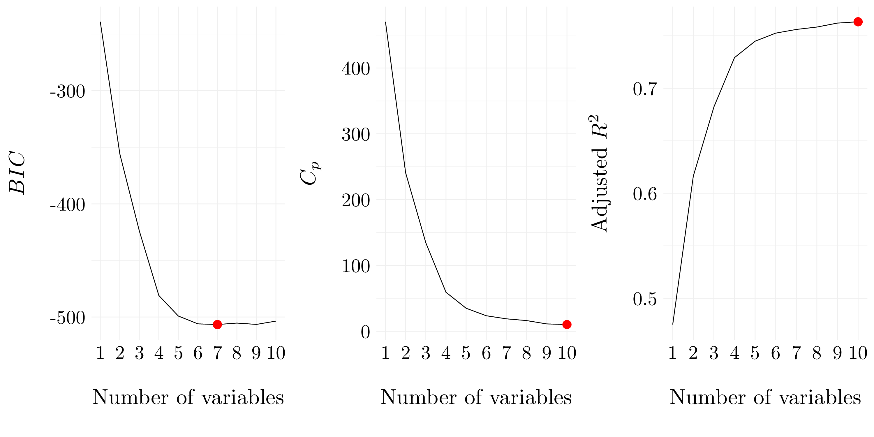
Figure 7.18: Best models according to \(C_p\), \(BIC\) and adjusted \(R^2\) for forward selection.

Table 7.1: Coefficients for the best model according to \(BIC\).
(Intercept)	PrivateYes	Top10perc	Room.Board	PhD	perc.alumni	Expend	Grad.Rate
-3295.056	2554.948	21.75788	1.18555	28.6945	41.16226	0.16548	21.72396

Table 7.2: Coefficients for the best model according to \(C_p\).
(Intercept)	PrivateYes	Apps	Accept	Top10perc	F.Undergrad	Room.Board	PhD	perc.alumni	Expend	Grad.Rate
-2959.954	2481.64	-0.18079	0.59595	26.94416	-0.1486	1.1412	26.30114	45.48378	0.16667	17.13799

Table 7.3: Coefficients for the best model according to Adjusted \(R^2\).
(Intercept)	PrivateYes	Apps	Accept	Top10perc	F.Undergrad	Room.Board	PhD	perc.alumni	Expend	Grad.Rate
-2959.954	2481.64	-0.18079	0.59595	26.94416	-0.1486	1.1412	26.30114	45.48378	0.16667	17.13799

According to BIC, a satisfactory model that uses just a subset of the predictors contatins the variables Private, Top10perc, Room.Board, PhD, perc.alumni, Expend and Grad.Rate.

Question (b)

Let’s a GAM on the training data, using out-of-state tuition as the response and the features selected in the previous question as the predictors.

gam_model <- gam(Outstate ~ Private + ns(Top10perc, 4) + ns(Room.Board, 4) + 
                   ns(PhD, 4) + ns(perc.alumni, 4) + ns(Expend, 4) + ns(Grad.Rate, 4), data = train)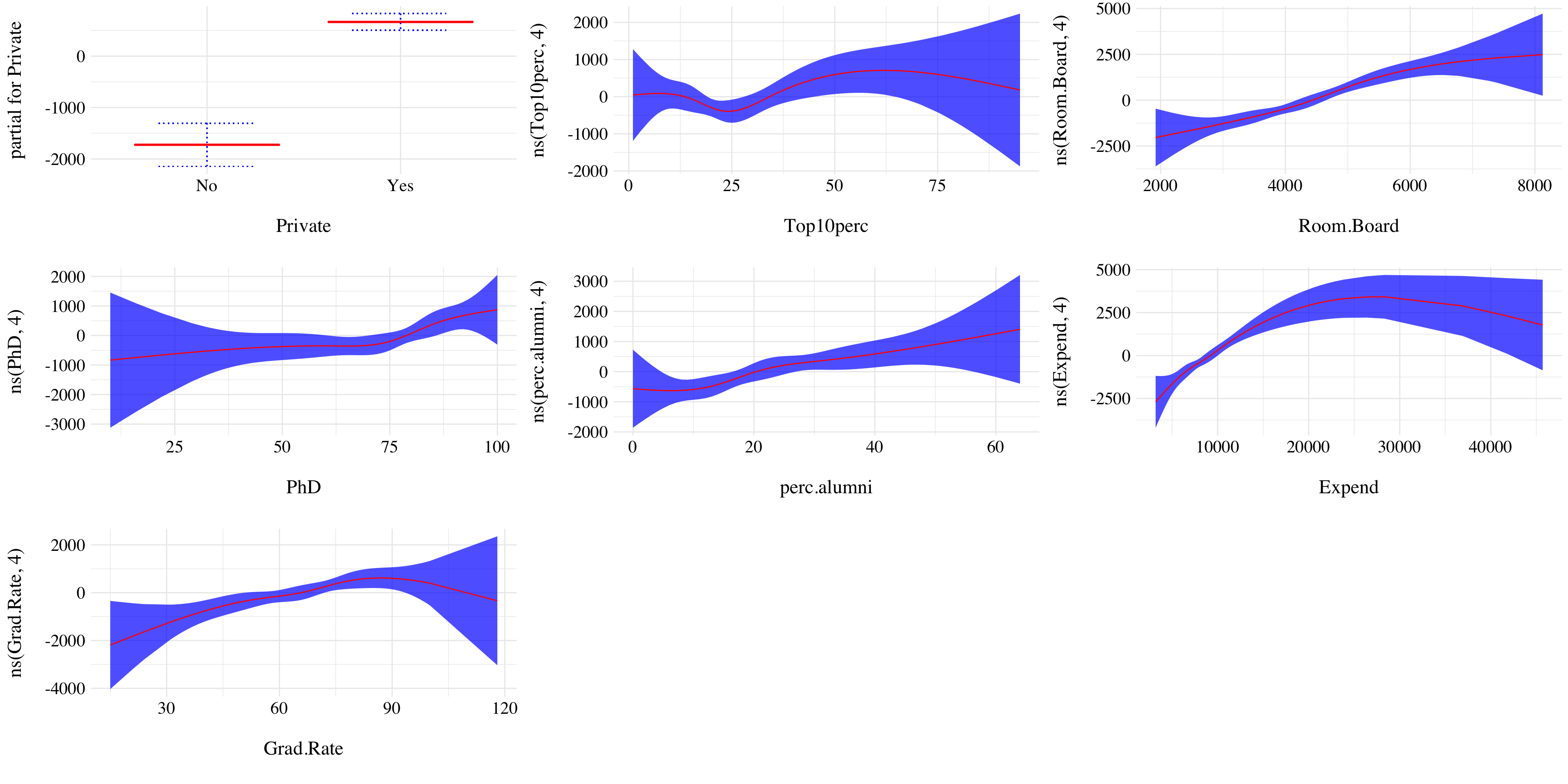

Figure 4.8: Results of the GAM.

We found the following results:

Private schools have higher of state tuition.
Universities that enroll the most students from top 10% of high school class appear to have slighly less tuition than the other ones.
The higher the room and board costs the higher the tuition.
The higher the number of PhD the higher the tuition.
The higher the percentage of alumni the higher the tuition.
The tuition is the highest for universities with not to low and not to high instructional expenditure per student.
The tuition appears to be almost linear with the graduation rate. The more we paid to enter the university the more likely we obtain the degree.
Question (c)

pred <- predict(gam_model, newdata = test, se.fit = TRUE)

We found out the GAM model have a MSE of 4.0899017^{6}. Let’s compare the results with a linear model.

lm_model <- lm(Outstate ~ ., data = train)
pred_lm <- predict(lm_model, newdata = test, se.fit = TRUE)

The MSE for the linear model is 4.2630381^{6}. So, the GAM model is significally better than the linear model.

Question (d)

According to the plots, most of the variables seems to have non-linear relationship with the response. Expend appears to be the variable with the most evidence of non-linear relationship with the response.

7.2.6 Exercise 11.

In Section 7.7, it was mentioned that GAMs are generally fit using a backfitting approach. The idea behind backfitting is actually quite simple. We will now explore backfitting in the context of multiple linear regression.

Suppose that we would like to perform multiple linear regression, but we do not have software to do so. Instead, we only have software to perform simple linear regression. Therefore, we take the following iterative approach: we repeatedly hold all but one coefficient esti- mate fixed at its current value, and update only that coefficient estimate using a simple linear regression. The process is continued until convergence — that is, until the coefficient estimates stop changing.

We now try this out on a toy example.

Question (a)

n <- 100
X1 <- rnorm(n)
X2 <- rnorm(n)
betas <- c(0.2, 0.3, -0.8)
Y <- betas[1] + betas[2] * X1 + betas[3] * X2 + rnorm(n, 0, 0.5)

Question (b)

Initialize \(\widehat{\beta}_1\) has a random value.

beta1_hat <- runif(1, 0, 1)

Question (c)

Assume \(\widehat{\beta}_1\) fixed, fit the model \[ Y - \widehat{\beta}_1X_1 = \beta_0 + \beta_2X_2 + \epsilon.\]

a <- Y - beta1_hat * X1
beta2_hat <- lm(a ~ X2)$coef[2]

Question (d)

Assume \(\widehat{\beta}_2\) fixed, fit the model \[ Y - \widehat{\beta}_2X_2 = \beta_0 + \beta_1X_1 + \epsilon.\]

a <- Y - beta2_hat * X2
beta1_hat <- lm(a ~ X1)$coef[2]

Question (e)

betas0 <- c(0)
betas1 <- c(beta1_hat)
betas2 <- c(beta2_hat)
for(i in 1:50){
  a <- Y - betas1[length(betas1)] * X1
  betas2 <- c(betas2, lm(a ~ X2)$coef[2])
  a <- Y - betas2[length(betas2)] * X2
  betas1 <- c(betas1, lm(a ~ X1)$coef[2])
  betas0 <- c(betas0, lm(a ~ X1)$coef[1])
}

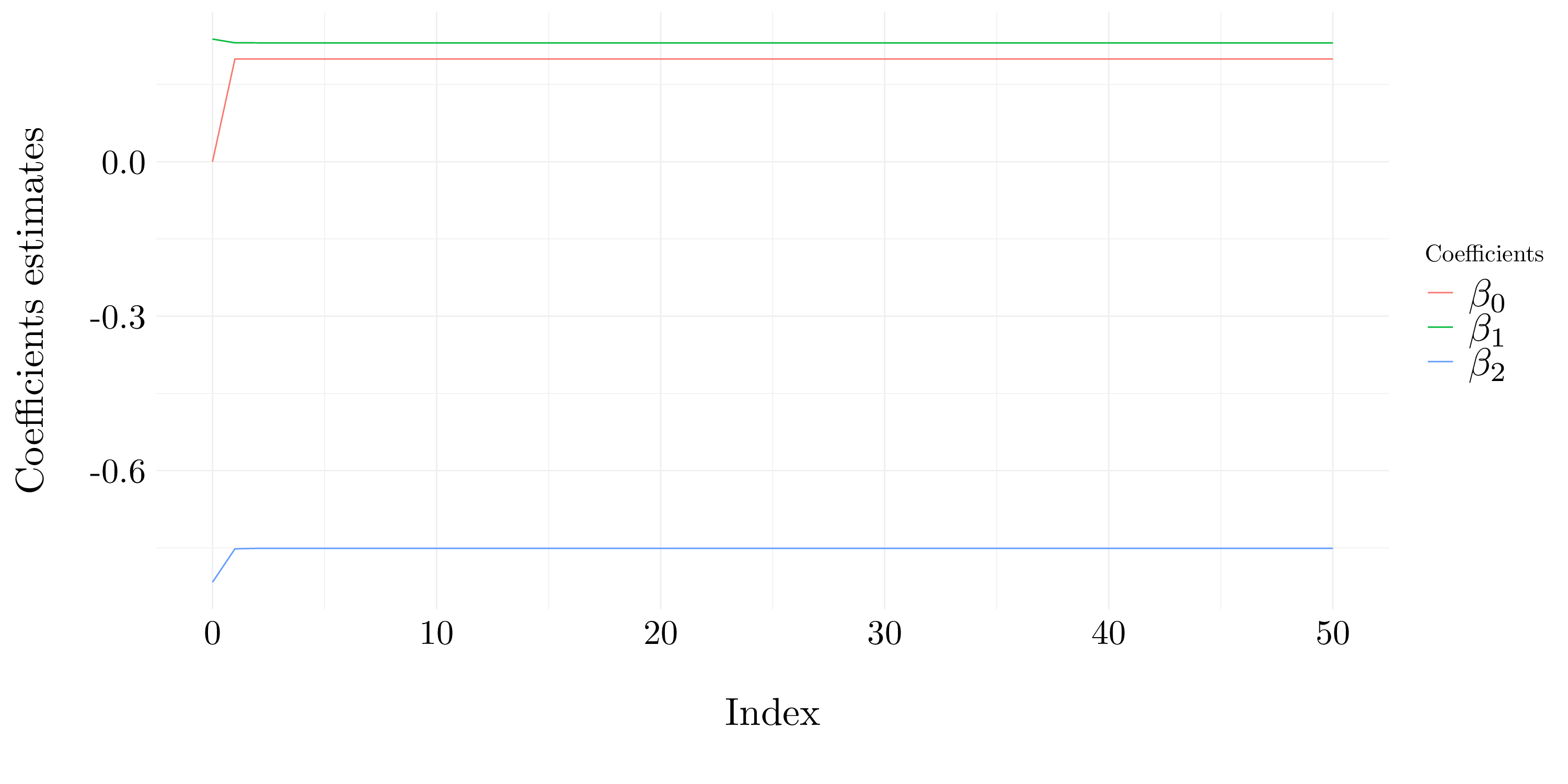
Figure 7.19: Estimation of the coefficients

Question (f)

Let’s perform a simple multiple linear regression and we’ll compare the results with the ones found in the previous answer.

lm_model <- lm(Y ~ X1 + X2)

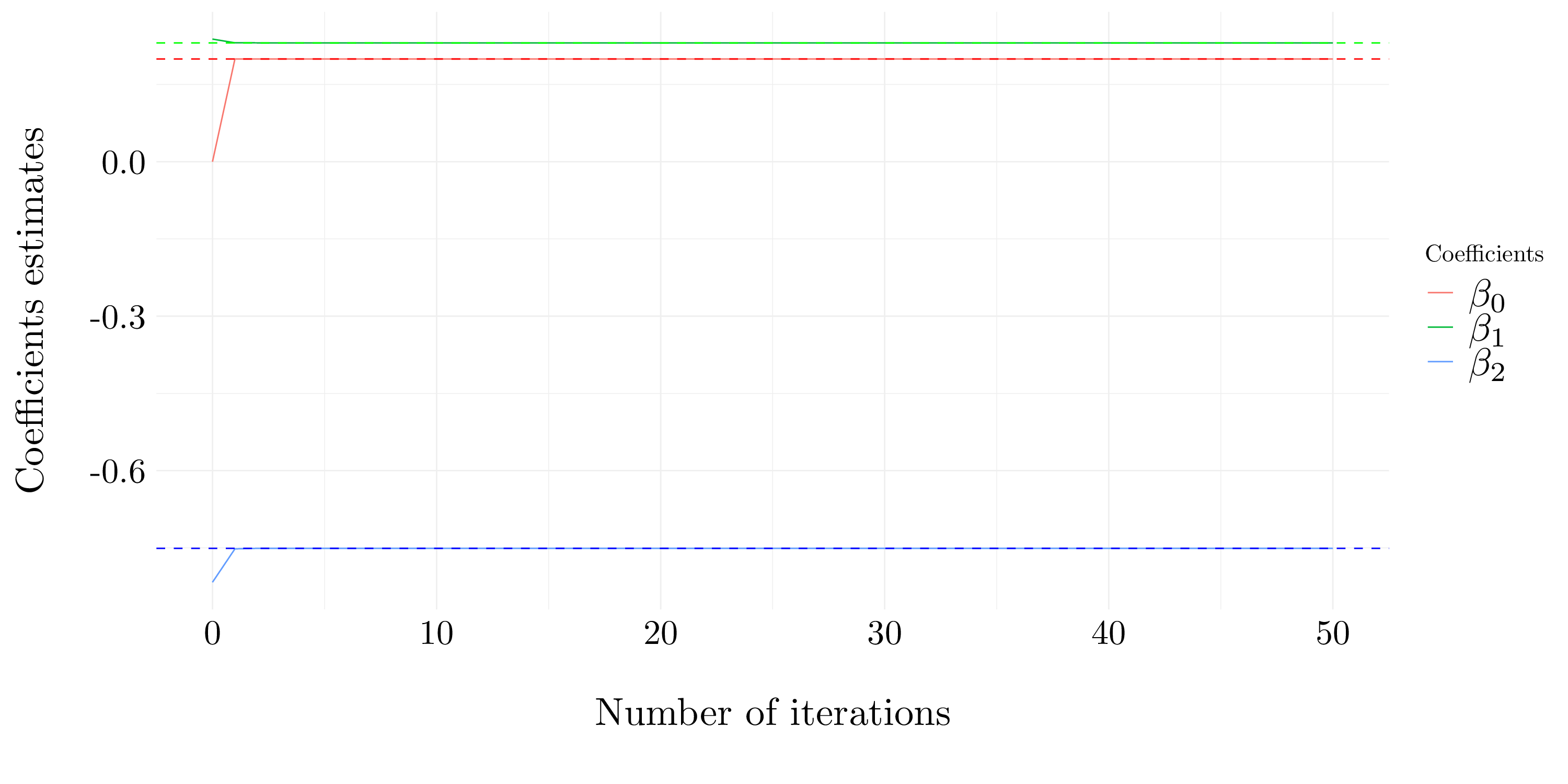
Figure 7.20: Estimation of the coefficients by lm

Question (g)

Two iterations seem to provide a rather good estimation of the coefficients. Moreover, after four iterations the algorithm appears to have converged.

7.2.7 Exercise 12.

This problem is a continuation of the previous exercise. In a toy example with \(p = 100\), show that one can approximate the multiple linear regression coefficient estimates by repeatedly performing simple linear regression in a backfitting procedure.

n <- 1000
p <- 100
X <- matrix(rnorm(n * p), ncol = p, nrow = n)
betas <- rnorm(p)
Y <- X %*% betas + rnorm(n, 0, 0.2)

d <- 50 # Number of iterations
betas_hat <- matrix(0, ncol = p, nrow = d)
MSE <- rep(0, d)
for(i in 1:d){
  for(j in 1:p){
      a <-  Y - (X[,-j] %*% betas_hat[i,-j])
      betas_hat[i:d, j] = lm(a ~ X[, j])$coef[2]
  }
  MSE[i] <- mean((Y - (X %*% betas_hat[i, ]))^2)
}

lm_model <- lm(Y ~ -1 + X)
betas_lm <- coef(lm_model)
MSE_lm <- mean((Y - (X %*% betas_lm))**2)

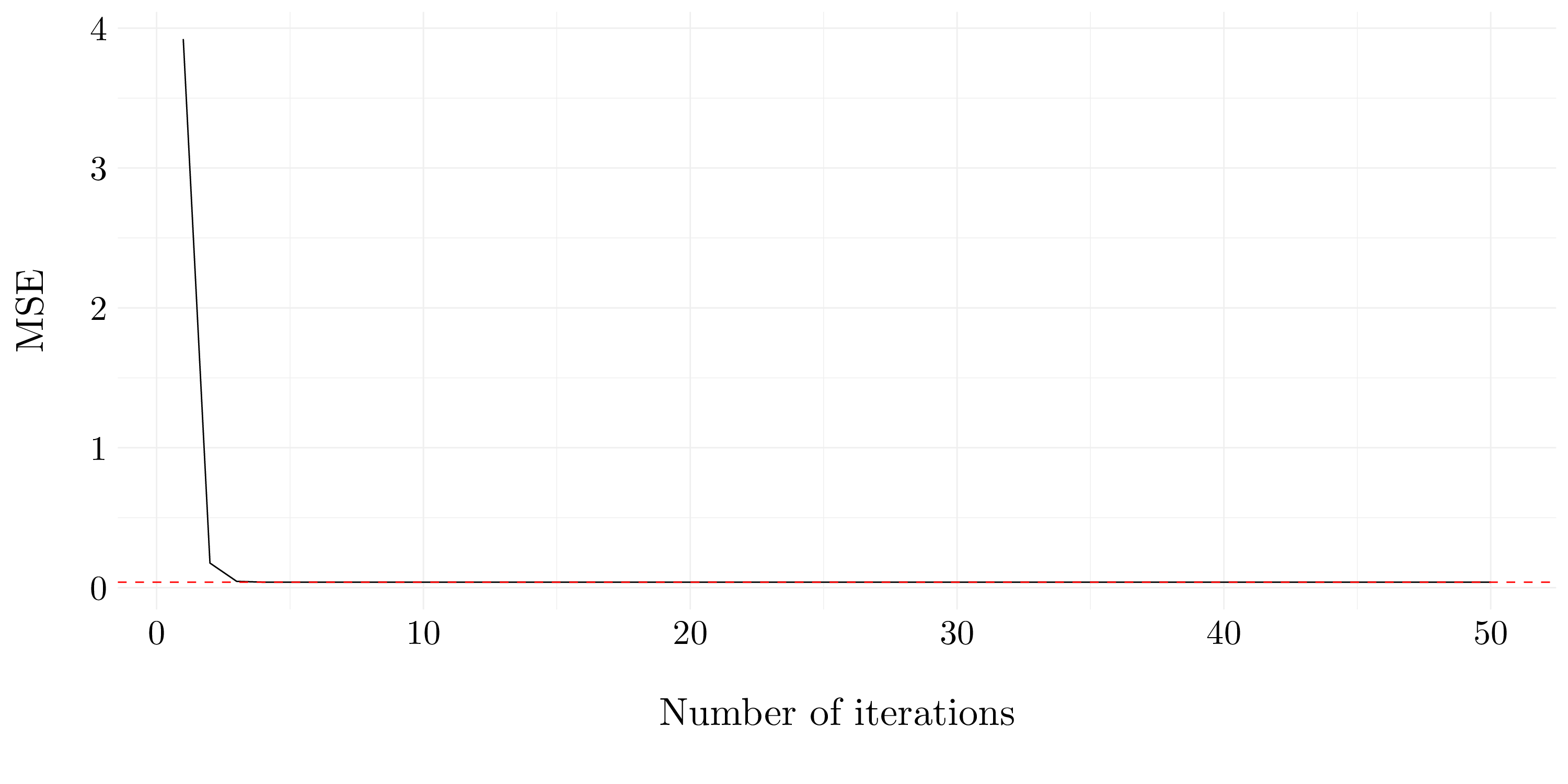
Figure 7.21: MSE using the backfitting approach compare to the lm model

After four iterations it appears that the backfiting approach has the same MSE than the linear model.