Introduction to funestim

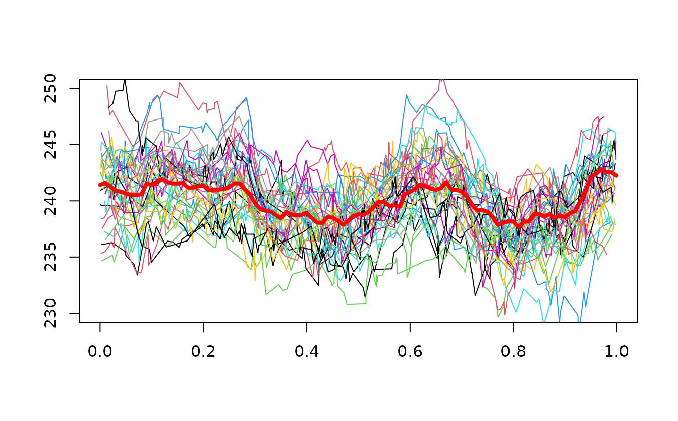
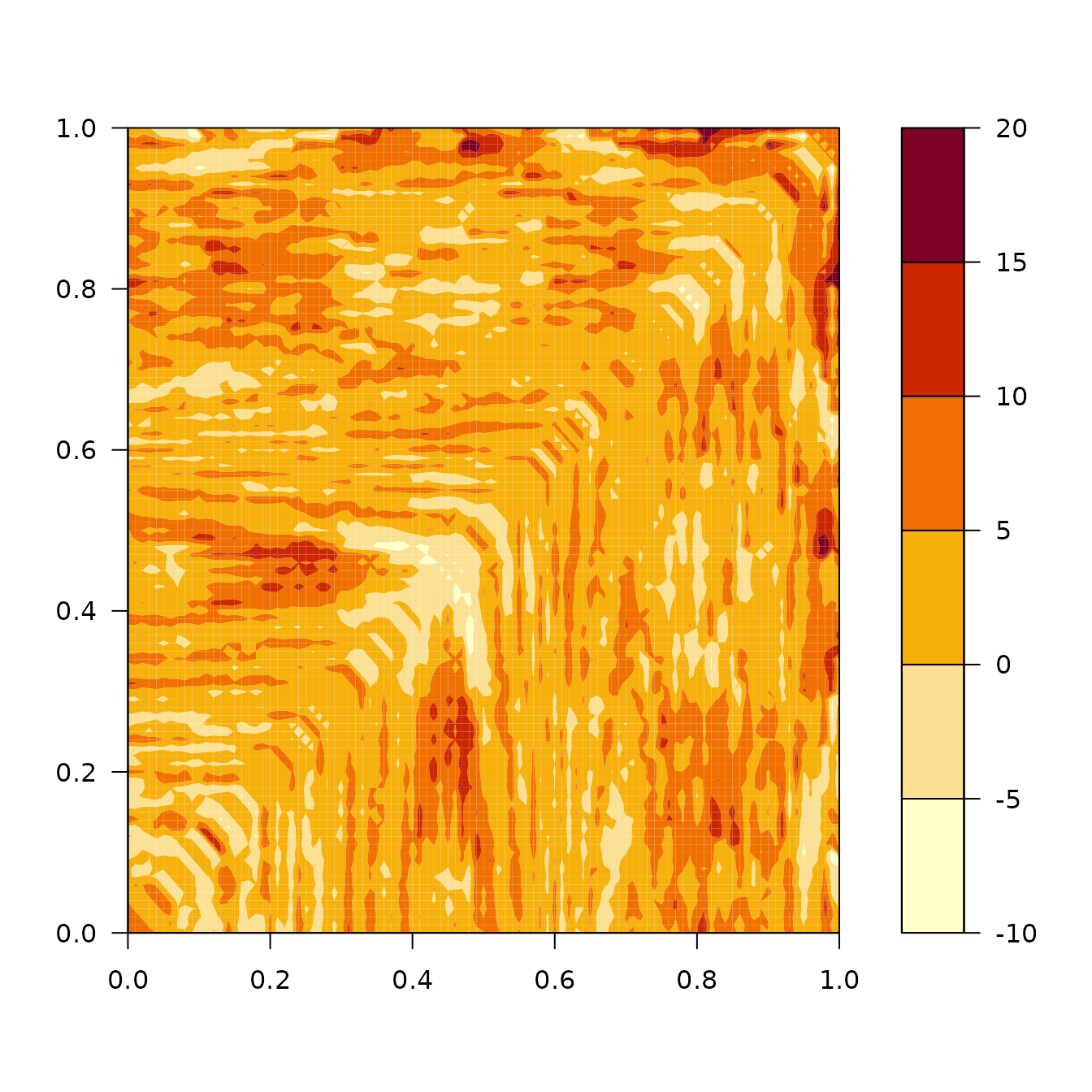
In this vignette, we will show how to estimate the mean and covariance functions of a functional dataset. For this example, we will use simulated data using the package simulater.

# Load the packages
library(funestim)
library(simulater)

First, we will generate some data.

mu <- learn_mean(powerconsumption)
cov <- learn_covariance(powerconsumption)
noise <- learn_noise(powerconsumption)

grid <- seq(0, 1, length.out = 101)
X <- generate_data(n = 100, m = 100, 
                   model_mean = mu, covariance = cov, 
                   model_noise = noise, 
                   lambda = exp(-5.5), 
                   ti = NULL, grid = grid,
                   p = 0.2, k = 1)

We perform an estimation of the mean curve.

obs_points <- seq(0, 1, length.out = 101)  # Estimation grid mean
band_points <- c(0.25, 0.5, 0.75) # Estimation grid regularity
delta_f <- function(m) exp(-log(m)**0.5)
mean_curve <- mean_ll(X, grid = obs_points,
                      grid_param = band_points, delta_f = delta_f)

We perform an estimation of the covariance surface.

obs_points <- seq(0, 1, length.out = 101)  # Estimation grid mean
band_points <- c(0.25, 0.5, 0.75) # Estimation grid regularity
delta_f <- function(m) exp(-log(m)**0.5)
cov_our <- covariance_ll(X, grid = obs_points, 
                         grid_param = band_points,
                         grid_bandwidth = NULL,
                         center = TRUE,
                         delta_f = delta_f,
                         n_obs_min = 2,
                         kernel_name = 'epanechnikov')

Steven Golovkine

2022-05-30